Building, Training, and Scaling Vision Transformers in TensorFlow
- Data Exploration - CIFAR-10
- Architecture
- Data Preprocessing for CIFAR-10
- Compiling and Training the Model
- Handling Larger Image Datasets
- Model Training on SageMaker
- Conclusion
The introduction of the Transformer architecture marked a significant milestone in the field of Natural Language Processing (NLP). The architecture was adaptable enough to find applications across many other fields of AI research, including Computer Vision. Vision Transformers (ViTs) were one of the earlier widely successful applications of Transformers outside of NLP, and they quickly achieved state-of-the-art on various image recognition tasks. The ViT applies the mechanism of self-attention to image patches. The trick was to adapt the tokenisation approach and treat these image patches as the model’s inputs. In fact, these image patches are passed through linear projections to obtain embeddings and enriched with positional encodings in a very similar way. These embeddings capture both feature and spatial information. ViTs are generally more data-hungry than traditional CNNs, as they have no inherent architectural inductive bias (such as locality or translation invariance). This means they typically require much more data to learn effective feature representations and, as such, thrive when pre-trained on large datasets.
Following a structure similar to my previous post on Transformers, we’ll run through the essential components of the Vision Transformer, describing their individual functions and explaining how to implement them as TensorFlow layers.
To put the model to use, we’ll look at an image classification task using the publicly accessible CIFAR-10 dataset. This is a dataset of 60000 32x32 3-channel images across 10 classes. It’s worth noting there is no imbalance across this dataset, so the ViT will have 6000 images of each class to work with.
The goal will be to make the architecture configurable and adapt it to different input image sizes, class counts, regularisation, patch, and layer configurations.
In researching the content for this post, I also explored larger-scale model training using the iNaturalist17 dataset. This dataset is considerably bigger, with more training instances, more classes and significant class imbalance. More consideration must be put towards data preparation for a dataset of this scale for training a ViT classifier. I will touch on some practical tips for dealing with large image datasets and some cloud tools to help manage training.
Before we jump in, definitely give the paper a read:
An Image is Worth 16x16 Words: Transformers for Image Recognition at Scale by Dosovitskiy et al., 2020.
Data Exploration - CIFAR-10
We’ll take a smaller dataset for data exploration and experimenting with the ViT architecture. This dataset is CIFAR-10, a collection of 60,000 colour images with 10 classes (6k images per class, images are 32x32 in RGB format). There are 50,000 training and 10,000 test images.
import tensorflow_datasets as tfds
import matplotlib.pyplot as plt
import os

os.environ["NO_GCE_CHECK"] = "true"

# Load dataset
dataset, info = tfds.load("cifar10", with_info=True, as_supervised=True, data_dir="~/tensorflow_datasets/")
train_dataset, test_dataset = dataset["train"], dataset["test"]

# CIFAR-10 label names
label_names = info.features["label"].int2str

# Display a few images, these are stored as image tensors with shape (32, 32, 3) / (height, width, channels)
plt.figure(figsize=(10, 5))
for i, (image, label) in enumerate(train_dataset.take(5)):
    plt.subplot(1, 5, i+1)
    plt.imshow(image)
    plt.title(label_names(label))
    plt.axis('off')
plt.show()
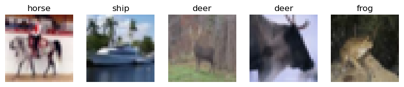
A sample of the first 5 images of the dataset.
Architecture
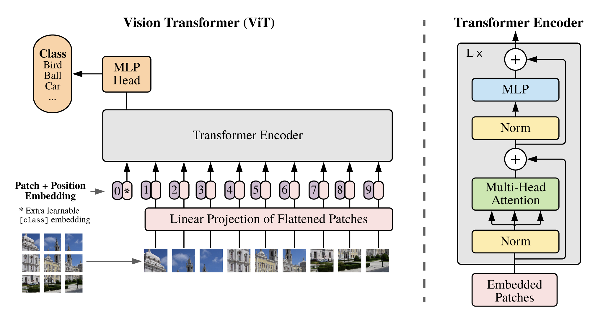
Figure 1: Vision Transformer Architecture, reproduced from “An Image is Worth 16x16 Words: Transformers for Image Recognition at Scale” by Dosovitskiy et al., 2020.
The ViT architecture builds on the original Transformer architecture. Let’s put together a high-level outline of the main implementation steps outlined in this diagram:
- Reshape the input image into a sequence of flattened 2d patches.
- Pass the flattened patches through a trainable linear projection to obtain D dimensions. This output is called the patch embeddings. Then, prepend/concatenate a learnable [class] token to the entire sequence of patch embeddings.
- Add the positional embedding (element-wise) to each patch embedding to represent the patch position in the sequence (learnable 1D embeddings).
- Pass the embedded patches through the transformer encoder, which consists of multiple layers of multi-head attention and MLP blocks. The encoder is slightly modified, moving the layer normalisation before the multi-head self-attention and MLP layers (see the above diagram).
- Pass the encoder output for the [class] token embedding to a classification head (feed-forward MLP) to obtain the class probabilities (using softmax). Before passing through the classification head, the output may pass through another normalisation layer.
- Assemble the individual layers into a complete Keras model.
The encoder applies self-attention across the patch embeddings and the [class] token. The [class] token interacts with all patch embeddings, learning to aggregate global information about the image as the encoder processes the sequence.
The encoder output corresponding to the [class] token is fed through an optional normalisation layer, followed by a classification head (an MLP using GELU activations). Depending on whether pre-training the model or fine-tuning it, the MLP:
- During pretraining: is a two-layer feed-forward network with one hidden layer and one linear layer (to enable more expressive learning).
- During fine-tuning: is a single linear layer (reducing complexity, to avoid over-fitting on smaller datasets).
We will run through each of these steps in more detail below.
1. Reshape and Flatten Images
This first step involves reshaping each input image into a sequence of flattened 2D patches. The layers will be designed flexibly, handling variable image input sizes and configurable patch sizes.
import tensorflow as tf

class PatchConverter(tf.keras.layers.Layer):
    def __init__(self, patch_size, **kwargs):
        super().__init__(**kwargs)
        self.patch_size = patch_size

    def call(self, images):
        batch_size = tf.shape(images)[0] # get shape of input image tensor and extract batch size
        patches = tf.image.extract_patches( # similar to applying a convolution, extracting patches from the image
            images=images,
            sizes=[1, self.patch_size, self.patch_size, 1],
            strides=[1, self.patch_size, self.patch_size, 1],
            rates=[1, 1, 1, 1], # sampling rate set to 1 (no dilation)
            padding="VALID"
        )
        patch_dim = patches.shape[-1] # last dimension of patches is the flattened patch size (e.g. 4x4 patches is 48 - 4x4x3)
        patches = tf.reshape(patches, [batch_size, -1, patch_dim]) # reshape patches into 3D tensor of shape [batch_size, total patches per image, flattened patch size]
        return patches
Using the CIFAR-10 image dimensions (32x32) and a patch size of 4 as an example, we use tf.image.extract_patches to extract a grid of 8x8 non-overlapping patches for each image. Each patch contains 4x4x3=48 values. The output here is a 4D tensor of shape [batch_size, 8, 8, 48]. Though the ViT expects a sequence of flattened patches, tf.reshape converts this grid of patches to a sequence with shape [batch_size, 64, 48] to be used for the next step, the patch embedding layer.
2. Patch Embeddings Through Linear Projection With Class Token
The next step in the process is to pass the sequence of flattened patches through a linear projection layer to obtain D-dimensional vectors. These fixed-size embeddings allow the ViT to handle input images of any size. With these patch embeddings, we can prepend a learnable [class] token that will aggregate information from all patches and will be used by the classification head later.
Through self-attention, the [class] token will attend to all other patch embeddings as it passes through multiple encoder layers, ultimately becoming a global representation of the entire image. The role of the classification head is to properly interpret this representation to predict the class label. The Q, K and V matrices in each attention head determine how each patch attends to other patches in the sequence. As these are optimised during training through gradient descent, the [class] token learns to better aggregate information from the most relevant patches to improve classification accuracy.
class PatchEmbeddingWithClassToken(tf.keras.layers.Layer):
    def __init__(self, embedding_dim, **kwargs):
        super().__init__(**kwargs)
        self.embedding_layer = tf.keras.layers.Dense(embedding_dim) # a simple dense layer for projection
        self.class_token = self.add_weight(
            shape=(1, 1, embedding_dim),
            initializer="random_normal",
            trainable=True,
            name="class_token"
        )

    def call(self, patches):
        patch_embeddings = self.embedding_layer(patches)
        batch_size = tf.shape(patch_embeddings)[0]
        class_token = tf.broadcast_to(self.class_token, [batch_size, 1, self.class_token.shape[-1]]) # duplicate class_token to match batch size
        return tf.concat([class_token, patch_embeddings], axis=1)
3. Positional Embedding Layer
Like Transformers, Vision Transformers don’t preserve the inherent position of each patch within the sequence, so we similarly enrich the embeddings with the positional information. These positional embeddings will be learnable, allowing the ViT to self-adapt to differing sequence lengths.
class PositionalEmbedding(tf.keras.layers.Layer):
    def __init__(self, num_patches, embedding_dim, **kwargs):
        super().__init__(**kwargs)
        self.position_embeddings = self.add_weight(
            shape=(1, num_patches, embedding_dim),
            initializer="random_normal",
            trainable=True,
            name="positional_embeddings"
        )

    def call(self, patch_embeddings):
        embeddings = self.position_embeddings + patch_embeddings
        return embeddings
4. Transformer Encoder Block
The encoder of the ViT is very similar to the encoder proposed in the original Transformer paper. The only adjustment involves moving the layer normalisation before the multi-head self-attention and MLP layers. We can stack this layer multiple times to create a deep Transformer encoder. We will similarly apply dropout to both the attention mechanism itself and the final output of the feed-forward network for extra regularisation.
Dropout within the attention mechanism plays a similar role to dropout applied across a fully connected network; it reduces over-reliance on specific portions of the input for improved generalisation. This means some of the attention weights are randomly zeroed out, and relationships between the patches (or tokens in the case of regular Transformers) are temporarily ignored during training. Attention is spread across the inputs more evenly, and overfitting is mitigated.
Masking Note: Unlike sequence processing tasks typically handled by Transformer architectures, Vision Transformers have no need for padding or causal masks. This is because patch sequence lengths within the image batch are always the same, and they don’t have any inherent sequential order, allowing each patch to attend to every other patch.
class EncoderLayer(tf.keras.layers.Layer):
    def __init__(self, num_heads, embedding_dim, mlp_dim, dropout_rate=0.1, **kwargs):
        super().__init__(**kwargs)
        self.attn_layer = tf.keras.layers.MultiHeadAttention(
            num_heads=num_heads, key_dim=embedding_dim // num_heads, dropout=dropout_rate
        )
        self.norm1 = tf.keras.layers.LayerNormalization()
        self.norm2 = tf.keras.layers.LayerNormalization()
        self.mlp = tf.keras.Sequential([ # can consider dropout after each of these Dense layers too (try if overfitting)
            tf.keras.layers.Dense(mlp_dim, activation="gelu"), # paper user GELU activation
            tf.keras.layers.Dense(embedding_dim)
        ])
        self.dropout = tf.keras.layers.Dropout(dropout_rate)

    def call(self, inputs, training=False):
        # mutli-head attention sublayer
        x = self.norm1(inputs)
        x = self.attn_layer(x, value=x, training=training)
        x = self.dropout(x, training=training)
        x = tf.keras.layers.Add()([x, inputs])

        # mlp sublayer
        x1 = self.norm2(x)
        x1 = self.mlp(x1)
        x1 = self.dropout(x1, training=training)
        x1 = tf.keras.layers.Add()([x1, x])

        return x1
5. Classification Head
The class token can now be passed through a classification head to obtain final class probabilities. The paper mentions the following:
“The classification head is implemented by a MLP with one hidden layer at pre-training time and by a single linear layer at fine-tuning time.” — Dosovitskiy et al. (2020)
Though we may not use this, the layer can be designed flexibly to easily accommodate both.
class ClassificationHead(tf.keras.layers.Layer):
    def __init__(self, num_classes, mlp_dim=None, **kwargs):
        super().__init__(**kwargs)
        output_layer = tf.keras.layers.Dense(num_classes, activation="softmax")
        if mlp_dim:
            self.mlp = tf.keras.Sequential([
                tf.keras.layers.Dense(mlp_dim, activation="gelu"),
                output_layer
            ])
        else:
            self.mlp = output_layer

    def call(self, class_token):
        return self.mlp(class_token)
6. Model Assembly
We can construct the Vision Transformer using these layers, where input sizes, patch sizes, number of encoder stacks, and embedding dimensions are all configurable (allowing flexible use with different datasets and image sizes). There are a few things to note, however:
- As suggested in the paper, we can apply layer normalisation to the class token embedding prior to passing it through the classification head.
- Tensorflow only determines the shapes when data is passed through the model
callmethod. Therefore, we can rely on the explicit formula to know the value ofnum_patchesfor thePositionalEmbeddinglayer (see below). Alternatively, the Tensorflow layerbuildmethod can initialise the layer weights based on the input size, which is called the first time the layer processes data. Typical implementation for ViTs assumes square images, simplifying patch conversion and calculations for positional encoding (ensure input images are square if using this ViT).
$\text{num_patches} = \left( \frac{\text{image_height}}{\text{patch_size}} \right) \times \left( \frac{\text{image_width}}{\text{patch_size}} \right) + 1$
class ViT(tf.keras.Model):
    def __init__(
        self,
        input_shape,
        patch_size,
        num_classes,
        embedding_dim,
        num_heads,
        num_layers,
        mlp_dim,
        dropout_rate,
        **kwargs
    ):
        super().__init__(**kwargs)
        self.patch_converter = PatchConverter(patch_size)
        self.patch_embedding_class_token = PatchEmbeddingWithClassToken(embedding_dim)
        self.positional_embedding = PositionalEmbedding(
            num_patches=(input_shape[0] // patch_size) ** 2 + 1, # +1 includes [class] embedding
            embedding_dim=embedding_dim
        )
        self.encoder_stack = [
            EncoderLayer(num_heads, embedding_dim, mlp_dim, dropout_rate)
            for _ in range(num_layers)
        ]
        self.class_token_norm = tf.keras.layers.LayerNormalization()
        self.classification_head = ClassificationHead(num_classes)


    def call(self, inputs):
        # Extract the patches and create the patch embeddings w/ class token
        patches = self.patch_converter(inputs)
        embeddings = self.patch_embedding_class_token(patches)

        # Add positional embeddings
        embeddings = self.positional_embedding(embeddings)

        # Encoder stack
        x = embeddings
        for layer in self.encoder_stack:
            x = layer(x)

        # Extract and normalize the [class] token
        class_token = x[:, 0]
        norm_class_token = self.class_token_norm(class_token)

        # Classification head
        class_probas = self.classification_head(norm_class_token)

        return class_probas
Layer Output Shape Tests
We can add some quick tests to ensure the output shape of each layer is correct for a single CIFAR-10 training image.
def test_transformer_layer_output_shapes(image):
    input_shape = (32, 32, 3) # image.shape[1:] without batch dim
    patch_size = 4
    embedding_dim = 64
    num_patches = (input_shape[0] // patch_size) ** 2 + 1
    num_heads = 4
    mlp_dim = 128
    dropout_rate = 0.1
    num_classes = 10

    # Patch Conversion
    patch_converter = PatchConverter(patch_size)
    patches = patch_converter(single_image)
    assert patches.shape == (1, 64, 48)

    # Patch Embeddings + Class Token
    patch_embedding_with_class_token = PatchEmbeddingWithClassToken(embedding_dim)
    embeddings = patch_embedding_with_class_token(patches)
    assert embeddings.shape == (1, 65, 64)
    assert num_patches == embeddings.shape[1]

    # Positional Embeddings
    positional_embedding = PositionalEmbedding(num_patches, embedding_dim)
    embeddings = positional_embedding(embeddings)
    assert embeddings.shape == (1, 65, 64)

    # Single Encoder Layer
    single_encoder = EncoderLayer(num_heads, embedding_dim, mlp_dim, dropout_rate)
    encoder_output = single_encoder(embeddings)
    assert encoder_output.shape == (1, 65, 64)

    # Class Token Norm & Classification Head
    class_token_norm = tf.keras.layers.LayerNormalization()
    classification_head = ClassificationHead(num_classes)
    class_token = encoder_output[:, 0]
    norm_class_token = class_token_norm(class_token)
    class_probas = classification_head(norm_class_token)
    assert class_probas.shape == (1, 10)

for image, label in train_dataset.take(1):
    single_image = tf.expand_dims(image, axis=0) # add a batch dimension
    print(f"Image shape: {single_image.shape}, Label: {label_names(label)}")
    test_transformer_layer_output_shapes(single_image)
    print("Tests passed!")
Image shape: (1, 32, 32, 3), Label: horse
Tests passed!
Data Preprocessing for CIFAR-10
Using TFDS, the CIFAR-10 dataset is already split, though we can apply further preprocessing. It’s worth noting that Transformer models have fewer inductive biases than ResNets or other CNNs, so they will initially require more training data. CIFAR-10 is a small dataset but well-suited for testing and experimentation. For the best performance, these models should be pre-trained on larger datasets (ImageNet, for example). Further preprocessing we will apply to the CIFAR-10 dataset include:
- Normalising/standardising the input image.
- Splitting the training set further to obtain a validation set.
- Configuring shuffling, batching and prefetching.
Later in this post, we will explore further preprocessing tasks, such as data augmentation, which will be a relevant step when working with larger datasets and trying to combat overfitting.
def normalize_image(image, label):
    image = tf.cast(image, tf.float32) / 127.5 - 1.0 # normalize to [-1, 1]
    return image, label

# load the training, validation and test sets
train_set = tfds.load("cifar10", split="train[:90%]", as_supervised=True, data_dir="~/tensorflow_datasets/") # 45,000 examples
valid_set = tfds.load("cifar10", split="train[90%:]", as_supervised=True, data_dir="~/tensorflow_datasets/") # 5,000 examples
test_set = tfds.load("cifar10", split="test", as_supervised=True, data_dir="~/tensorflow_datasets/") # 10,000 examples

# shuffle, batch and prefetch
batch_size = 128
train_set = train_set.map(normalize_image).shuffle(1000).batch(batch_size).prefetch(tf.data.AUTOTUNE)
valid_set = valid_set.map(normalize_image).batch(batch_size).prefetch(tf.data.AUTOTUNE)
test_set = test_set.map(normalize_image).batch(batch_size).prefetch(tf.data.AUTOTUNE)

for images, labels in train_set.take(1):
    print(f"Shape of images in first batch: {images.shape}, with labels: {labels.shape}")
Shape of images in first batch: (128, 32, 32, 3), with labels: (128,)
Compiling and Training the Model
Before constructing the model, compiling it and fitting it, we can prepare a few callbacks:
- A checkpoint callback to ensure the best-performing model weights (in terms of validation loss) are saved.
- An early stopping callback to ensure training stops when the validation performance stops improving, preventing overfitting and reducing wasteful use of computing resources.
import time

# prep callbacks
checkpoint_callback = tf.keras.callbacks.ModelCheckpoint(
    "checkpoints/vit_cifar10_saturncloud/vit_cifar10_epoch-{epoch:02d}.weights.h5",
    save_weights_only=True,
    save_best_only=True,
    monitor="val_loss",
    mode="min",
    verbose=1
)

early_stopping_callback = tf.keras.callbacks.EarlyStopping(
    patience=5,
    restore_best_weights=True,
)

# create ViT
vit_cifar10_model = ViT(
    input_shape=(32, 32, 3),
    patch_size=4,
    num_classes=10,
    embedding_dim=64,
    num_heads=4,
    num_layers=4,
    mlp_dim=128,
    dropout_rate=0.1,
)

# compile
vit_cifar10_model.compile(
    optimizer=tf.keras.optimizers.Adam(learning_rate=3e-4),
    loss=tf.keras.losses.SparseCategoricalCrossentropy(),
    metrics=['accuracy']
)

start_time = time.time()

# train
vit_cifar10_model.fit(
    train_set,
    validation_data=valid_set,
    epochs=30,
    callbacks=[checkpoint_callback]
)

end_time = time.time()
total_time = end_time - start_time
print(f"Total training time for 30 epochs: {total_time:.2f} seconds ({total_time / 60:.2f} minutes)")
Here, the model has trained to a modest ~63% validation accuracy in 30 epochs (roughly 4.5 minutes of training locally).
Epoch 1/30
352/352 ━━━━━━━━━━━━━━━━━━━━ 0s 37ms/step - accuracy: 0.2793 - loss: 1.9829
Epoch 1: val_loss improved from inf to 1.58398, saving model to checkpoints/vit_cifar10_saturncloud/vit_cifar10_epoch-01.weights.h5
352/352 ━━━━━━━━━━━━━━━━━━━━ 33s 49ms/step - accuracy: 0.2795 - loss: 1.9825 - val_accuracy: 0.4188 - val_loss: 1.5840
Epoch 2/30
352/352 ━━━━━━━━━━━━━━━━━━━━ 0s 21ms/step - accuracy: 0.4484 - loss: 1.5165
Epoch 2: val_loss improved from 1.58398 to 1.30431, saving model to checkpoints/vit_cifar10_saturncloud/vit_cifar10_epoch-02.weights.h5
352/352 ━━━━━━━━━━━━━━━━━━━━ 8s 22ms/step - accuracy: 0.4485 - loss: 1.5163 - val_accuracy: 0.5288 - val_loss: 1.3043
Epoch 3/30
352/352 ━━━━━━━━━━━━━━━━━━━━ 0s 21ms/step - accuracy: 0.5369 - loss: 1.2803
Epoch 3: val_loss improved from 1.30431 to 1.20400, saving model to checkpoints/vit_cifar10_saturncloud/vit_cifar10_epoch-03.weights.h5
352/352 ━━━━━━━━━━━━━━━━━━━━ 8s 22ms/step - accuracy: 0.5370 - loss: 1.2802 - val_accuracy: 0.5546 - val_loss: 1.2040
Epoch 4/30
352/352 ━━━━━━━━━━━━━━━━━━━━ 0s 21ms/step - accuracy: 0.5760 - loss: 1.1724
Epoch 4: val_loss improved from 1.20400 to 1.15570, saving model to checkpoints/vit_cifar10_saturncloud/vit_cifar10_epoch-04.weights.h5
352/352 ━━━━━━━━━━━━━━━━━━━━ 8s 22ms/step - accuracy: 0.5761 - loss: 1.1723 - val_accuracy: 0.5896 - val_loss: 1.1557
Epoch 5/30
351/352 ━━━━━━━━━━━━━━━━━━━━ 0s 21ms/step - accuracy: 0.6092 - loss: 1.0831
Epoch 5: val_loss improved from 1.15570 to 1.11848, saving model to checkpoints/vit_cifar10_saturncloud/vit_cifar10_epoch-05.weights.h5
352/352 ━━━━━━━━━━━━━━━━━━━━ 8s 22ms/step - accuracy: 0.6092 - loss: 1.0830 - val_accuracy: 0.5994 - val_loss: 1.1185

...

Epoch 28/30
351/352 ━━━━━━━━━━━━━━━━━━━━ 0s 21ms/step - accuracy: 0.8909 - loss: 0.3027
Epoch 28: val_loss did not improve from 1.03000
352/352 ━━━━━━━━━━━━━━━━━━━━ 8s 22ms/step - accuracy: 0.8909 - loss: 0.3027 - val_accuracy: 0.6318 - val_loss: 1.5248
Epoch 29/30
351/352 ━━━━━━━━━━━━━━━━━━━━ 0s 21ms/step - accuracy: 0.8976 - loss: 0.2840
Epoch 29: val_loss did not improve from 1.03000
352/352 ━━━━━━━━━━━━━━━━━━━━ 8s 22ms/step - accuracy: 0.8976 - loss: 0.2840 - val_accuracy: 0.6304 - val_loss: 1.6130
Epoch 30/30
352/352 ━━━━━━━━━━━━━━━━━━━━ 0s 21ms/step - accuracy: 0.8991 - loss: 0.2807
Epoch 30: val_loss did not improve from 1.03000
352/352 ━━━━━━━━━━━━━━━━━━━━ 8s 22ms/step - accuracy: 0.8992 - loss: 0.2807 - val_accuracy: 0.6330 - val_loss: 1.6445
Total training time for 30 epochs: 263.43 seconds (4.39 minutes)
Congratulations! You just built a Vision Transformer. Next, we’ll examine the architecture adjustments that can help better equip this model for larger datasets. We’ll also look at practical data preparation considerations for larger, imbalanced datasets.
Handling Larger Image Datasets
The iNaturalist 2017 dataset is a competition dataset with a total of 579,184 training images across 5089 classes (13 parent categories). The specifics of the data preparation can be found under inat17-pretraining/dataset-utils, though in summary:
- COCO-styled JSON annotation files are loaded and filtered, and category IDs are reassigned to make them sequential and subset-specific.
- Oversampling or undersampling is applied to balance the dataset and improve class balance for training (measures a normalised class distribution entropy against a desired threshold).
- Processed examples and updated category mappings are saved to disk in new JSON files.
- Low-frequency classes are flagged for augmentation and saved to a new JSON file.
- The processed JSON files are loaded, and dataset batches are built from the mapped filenames.
- Images are loaded, decoded and resized with padding, and a dedicated TensorFlow pipeline augments images (e.g. greyscale conversion, random rotations, zooms, flips) for the underrepresented class IDs, and these are added to the dataset.
- A final round of shuffling and validation ensures the final batch labels and filenames are correct.
This pipeline ensures the dataset is formatted correctly, batched, and balanced through augmentation and entropy-based sampling. The targeted augmentations also push the model to be more robust by encouraging it to learn generalisable features and avoid overfitting.
Architecture and Training Adjustments
Pretraining a Vision Transformer from scratch requires much larger datasets. Some key adjustments (as highlighted in the paper) can be made to ensure heavier regularisation. This will help combat overfitting, ensuring the model performs just as well on the test sets or any other unseen data. The architecture has also moved from a notebook to a single Python script under sagemaker/vision_transformer.py (used when creating training jobs on SageMaker, more on this later). The architecture updates include:
- Weight Decay: L2 weight decay is added as the kernel regulariser to all dense layers (in the embedding layer, encoder MLPs and the classification head).
- Updated Activations: GELU activation functions are used in the dense layers across the entire architecture (except, of course, within the final output layer of the classification head, which must use a softmax activation to produce class probabilities).
- Additional Hyperparameters: Additional configurable MLP dimension and weight decay hyperparameters are added to support the changes above.
In addition to the architecture changes, the following training changes were made (under sagemaker/train.py):
- Addressing Class Imbalance: The data preparation tasks outlined above aim to address the skewed class distribution. A weighted loss is also used as another measure to address this imbalance. Scikit-learn offers a handy function to compute these weights:
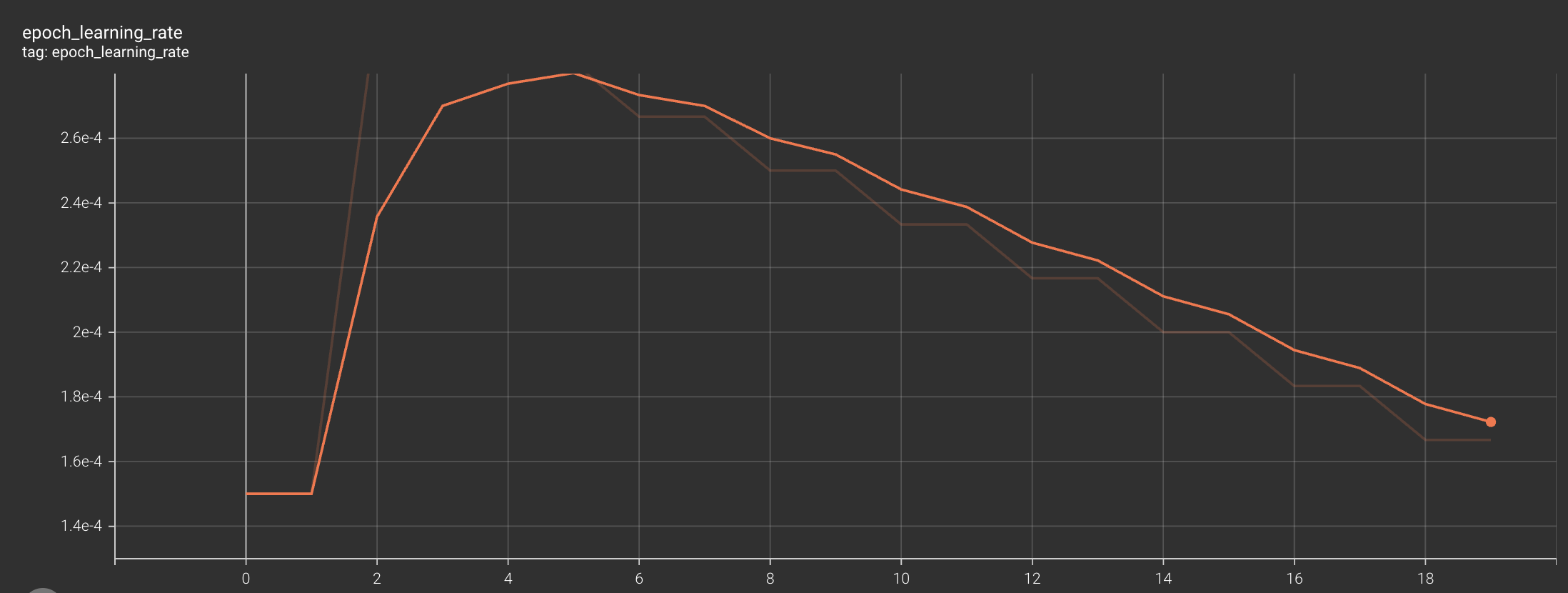
compute_class_weight. These weights are applied during model training and will give more importance to underrepresented classes. - Custom Learning Rate Scheduling (sagemaker/lr_schedule.py): Instead of using a constant learning rate, we can implement a custom learning rate scheduler that will include both a warmup phase and a linear decay. This approach can help keep training stabilised and can often lead to better convergence. A base learning rate can be set for the initial warmup to work up to before decay kicks in. See the TensorBoard screenshot below for a visual plot of the learning rate through training epochs.
- Model Checkpointing: It’s always good practice to save model checkpoints, at least when a metric such as the validation loss improves. This can allow you to resume training and select the best-performing model if an interruption occurs.
Model Training on SageMaker
Training models locally is great for quick experimentation and keeping costs low, but cloud environments offer many key advantages when scaling to larger datasets. Personally, I don’t have access to powerful GPUs locally, so using the cloud gives me easy access to GPU or TPU instances for faster, more efficient training. For many use cases, running a few training jobs incurs relatively low costs (at least cheaper than investing in similar hardware locally).
Cloud platforms also provide helpful tools for distributed training, experiment tracking, and deployment. I’ve primarily used AWS SageMaker to run jobs on GPU instances and track experiments, but Saturn Cloud is another helpful option, offering scalable resources for model training.
Let’s look at the basic setup required to get started with the SageMaker platform.
SageMaker Training Jobs
The training script (sagemaker/train.py in this case) can be set up to accept training hyperparameters via command-line arguments, allowing for flexible configuration when launching jobs and easy experimentation.
if __name__ == "__main__":
    parser = argparse.ArgumentParser()

    # model directory
    parser.add_argument('--model_dir', type=str)

    # hyperparameters
    parser.add_argument("--batch-size", type=int, default=16)
    parser.add_argument("--epochs", type=int, default=8)
    parser.add_argument("--base-learning-rate", type=float, default=1e-4)

    args = parser.parse_args()
    main(args)
Once your script is ready, launching a training job is as simple as configuring a sagemaker.tensorflow.TensorFlow estimator with the relevant settings. Calling fit on the estimator and providing the paths to your prepared training and validation datasets will start the job on AWS. Progress can be monitored via the SageMaker dashboard, and trained model artifacts will be saved to your S3 locations. Configuring an S3 path for TensorBoard logs is also useful, allowing you to visualise training and validation metrics over time (helpful for identifying issues like overfitting early in your experimentation).
The example below shows the SageMaker script used to launch the training job (sagemaker_script.py).
import sagemaker
from sagemaker.tensorflow import TensorFlow
from sagemaker.debugger import TensorBoardOutputConfig

train_data = "s3://inat17-train-val-records/train_val_images-processed(Aves)/train2017"
valid_data = "s3://inat17-train-val-records/train_val_images-processed(Aves)/val2017"
experiment_id = "exp4"
output_path = f"s3://inat17-vit-model-artifacts/{experiment_id}"


tensorboard_output_config = TensorBoardOutputConfig(
    s3_output_path=f"{output_path}/tensorboard",
    container_local_output_path="/opt/ml/output/tensorboard"
)

tf_estimator = TensorFlow(
    entry_point="train.py",
    source_dir="./sagemaker",
    role="arn:aws:iam::012345678901:role/SageMakerRoleViTTraining",
    instance_count=1,
    instance_type="ml.g4dn.2xlarge",
    framework_version="2.16",
    py_version="py310",
    hyperparameters={
        "batch-size": 32,
        "epochs": 20,
        "base-learning-rate": 3e-4,
    },
    output_path=output_path,
    checkpoint_s3_uri=f"{output_path}/checkpoints",
    tensorboard_output_config=tensorboard_output_config,
    volume_size=30,
    script_mode=True
)

# Launch training
tf_estimator.fit({
    "train": train_data,
    "valid": valid_data
})
Conclusion
Thanks for reading; the entire source code for this project can be found here. Feel free to reach out if you have any questions; my links are in the page footer.
👋