Implementing the Original Transformer Architecture in TensorFlow
- Architecture - Quick Overview
- Positional Encoding
- Masking
- Multi-Head Attention
- Encoder
- Decoder
- Output Projection Layer
- Final Thoughts
Hey! It’s been quite a while since my last post. Between then and now, I’ve also migrated content from my old site to this new one and, in the process, dropped a few old posts. I figured I’d break the long hiatus by writing about a groundbreaking research paper that introduced the Transformer architecture, which relies solely on attention mechanisms. These attention mechanisms (first introduced in an earlier paper in the context of sequence to sequence models) aimed to solve a significant limitation of RNNs at the time: short-term memory. Architectures like LSTMs or GRUs can typically handle only shorter sequences because representations of their inputs may be carried over many steps before they’re actually used. Attention mechanisms, however, align the decoder at each time step with the parts of the input sequence that are most relevant.
The Transformer architecture relies exclusively on these attention mechanisms (albeit through a more generalised approach), and as such, doesn’t suffer so much from the usual drawbacks associated with RNNs in many NLP tasks: vanishing/exploding gradients, longer training times, difficulty parallelising across many GPUs, and most importantly, limited ability to capture long-term patterns in input sequences.
Since its introduction, the Transformer has gone on to revolutionise many active fields of AI research, including computer vision (the Vision Transformer—ViT—is comparable in performance to CNNs for tasks such as image classification and object detection).
Anyway, the focus of this post will be a short breakdown of the essential components of this original 2017 architecture. If you haven’t already, I’d definitely recommend giving the paper a read first:
“Attention Is All You Need” by Vaswani et al., 2017
TIP There is a TensorFlow PluggableDevice to enable training on Mac GPUs called tensorflow-metal. If you’re using an Apple silicon chip like me, you can install this via
python3 -m pip install tensorflow-metal.
Architecture - Quick Overview
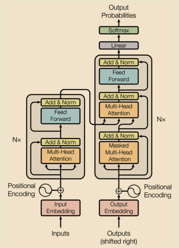
Figure 1: Transformer Architecture, reproduced from “Attention is All You Need” by Vaswani et al., 2017.
This diagram is pulled directly from the research paper. The architecture follows an encoder-decoder structure. Embeddings are created from the tokenized inputs for both the encoder and decoder, with positional encodings added to capture the order of tokens. These embeddings are then fed into their respective stacks. Finally, the output is passed through a dense layer with a softmax activation to produce a probability distribution. That’s the architecture in a nutshell. In the following sections, I’ll walk through each step in more detail.
I’ve chosen to only focus on the core components of the architecture, and so will omit the technical details of data preparation. A quick run through of these for an example NMT use case are:
- Loaded and shuffled the dataset of English to Spanish translations.
- Passed the sentences through
TextVectorizationlayers and inserted SOS and EOS tokens. - Prepared some training and validation sets (including splits for both the encoder and decoder inputs).
- Created embeddings from the tokenized inputs ids, with an embedding size of 128.
Now we can jump right into positional encoding.
Positional Encoding
Directly after creating embeddings, we want to construct a vector that encodes positional information for each token in a sequence. Sine and cosine functions of varying frequencies generate unique positional encodings that match the dimension of the embeddings. These positional vectors are then added to the token embeddings, allowing the model to recognize the order and relative positions of the tokens within the sequence.
class PositionalEncoding(tf.keras.layers.Layer):
    def __init__(self, max_length, embed_size, dtype=tf.float32, **kwargs):
        super(PositionalEncoding, self).__init__(dtype=dtype, **kwargs)

        # create the positional indices and scaling factors
        position_indices = np.arange(max_length)
        scaling_factors = 2 * np.arange(embed_size // 2)

        # create the positional embedding matrix
        pos_emb = np.zeros((1, max_length, embed_size))
        pos_emb[0, :, 0::2] = np.sin(position_indices[:, None] / (10_000 ** (scaling_factors / embed_size)))
        pos_emb[0, :, 1::2] = np.cos(position_indices[:, None] / (10_000 ** (scaling_factors / embed_size)))

        np_dtype = tf.as_dtype(dtype).as_numpy_dtype
        self.pos_encodings = tf.constant(pos_emb.astype(np_dtype))
        self.supports_masking = True

    def call(self, inputs):
        seq_len = tf.shape(inputs)[1]
        return inputs + self.pos_encodings[:, :seq_len, :]

pos_embed_layer = PositionalEncoding(max_length, embed_size)
encoder_in = pos_embed_layer(encoder_embeddings)
decoder_in = pos_embed_layer(decoder_embeddings)
Masking
We can manage the attention masks used by the MultiHeadAttention layer by setting up two masking layers:
- A padding mask, which will mask padding tokens in the input sequences for both the encoder and decoder.
- A causal mask, which will prevent the model from attending to future tokens.
NOTE Masking is only crucial within the attention layer and ensures the attention mechanism only attends to relevant tokens. The normalization and dense layers further up the stack do not require masks because their operations are uniform across all tokens. The
MultiHeadAttentionlayer has built in support for padding and causal masking, but I think it’s a helpful exercise to manage these yourself, to gain a deeper understanding of how the attention mechanism works.
# padding and causal masks
class PaddingMask(tf.keras.layers.Layer):
    def call(self, inputs):
        return tf.math.not_equal(inputs, 0)[:, tf.newaxis]

class CausalMask(tf.keras.layers.Layer):
    def __init__(self, **kwargs):
        super().__init__(**kwargs)
        self.supports_masking = True

    def call(self, inputs):
        seq_len = tf.shape(inputs)[1]
        return tf.linalg.band_part(tf.ones((seq_len, seq_len), tf.bool), -1, 0)

encoder_pad_mask = PaddingMask()(encoder_input_ids)
decoder_pad_mask = PaddingMask()(decoder_input_ids)

causal_mask = CausalMask()(decoder_embeddings)
Multi-Head Attention
The multi-head attention layers nested within the encoder and decoder stacks is where the model focuses on different parts of the input sequence simultaneously. The use of multiple attention heads allows the model to capture different relationships within the data, better understanding complex patterns and dependencies throughout the sequence. Here is how it works:
-
Input Embeddings: The input consists of a sequence of embeddings (which include positional encodings as described above).
-
Linear Projection: The input embedding matrix $X$ is projected into three different sets of lower-dimensional vectors: queries $Q$, keys $K$, and values $V$. This is done by multiplying $X$ by separate learned weight matrices: $Q = XW^Q, K = XW^K, V = XW^V$. Each attention head uses its own set of weight matrices, allowing different heads to focus on different characteristics of the sequence.
- Scaled Dot-Product Attention
- Similarity measures are computed $Q \cdot K^T$ resulting in a set of raw attention scores (for each key in the sequence). These are scaled (to combat tiny gradients) and passed through a softmax function $\text{softmax}(\frac{QK^T}{\sqrt{d_k}})$ producing a probability distribution, with scores now representing how much attention to give to each key’s corresponding value. This scaling factor can instead be a trainable parameter if setting
use_scale=True. - A weighted sum of the values is produced $\sum_{i}(\text{Attention Weight}_i \times V_i)$ by multiplying each value by its corresponding attention weight, and summing the results.
- Note, a masked multi-head attention layer will mask out some of these key/value pairs by adding a large negative value to the corresponding raw attention scores, prior to passing them to the softmax function.
- Similarity measures are computed $Q \cdot K^T$ resulting in a set of raw attention scores (for each key in the sequence). These are scaled (to combat tiny gradients) and passed through a softmax function $\text{softmax}(\frac{QK^T}{\sqrt{d_k}})$ producing a probability distribution, with scores now representing how much attention to give to each key’s corresponding value. This scaling factor can instead be a trainable parameter if setting
-
Attention Head Concatenation: A single tensor is produced by concatenating the outputs from each attention head along the depth dimension.
- Final Linear Projection: The concatenated output is passed through a final linear layer (with a learned weight matrix $W^O$). The output is a sequence of vectors, each of which has collected information from various portions of the input sequence (captured by the attention heads).
Encoder
The encoder comprises a stack of $N$ identical layers, each with two sublayers:
- First, a multi-head attention layer as described above.
- Second, a simple fully connected feed forward network.
Residual connections are applied around each sublayer, adding the sublayer’s input to its output, followed by layer normalization. For regularization, dropout is applied to the output of both sublayers prior to normalization.
class EncoderLayer(tf.keras.layers.Layer):
    def __init__(self, embed_size, att_heads, ff_units, dropout_rate, **kwargs):
        super().__init__(**kwargs)
        self.supports_masking = True
        self.attn_layer = tf.keras.layers.MultiHeadAttention(
            num_heads=att_heads, key_dim=embed_size, dropout=dropout_rate
        )
        self.norm1 = tf.keras.layers.LayerNormalization()
        self.norm2 = tf.keras.layers.LayerNormalization()
        self.ffn = tf.keras.Sequential([
            tf.keras.layers.Dense(ff_units, activation="relu"),
            tf.keras.layers.Dense(embed_size),
            tf.keras.layers.Dropout(dropout_rate)
        ])

    def call(self, inputs, mask=None):
        # multi-head attention sublayer
        attn_output = self.attn_layer(inputs, value=inputs, attention_mask=mask)
        out1 = self.norm1(tf.keras.layers.Add()([attn_output, inputs]))

        # fully connected sublayer
        ffn_output = self.ffn(out1)
        out2 = self.norm2(tf.keras.layers.Add()([ffn_output, out1]))

        return out2

N, att_heads, dropout_rate, ff_units = 2, 8, 0.1, 128
encoder_layers = [EncoderLayer(embed_size, att_heads, ff_units, dropout_rate) for _ in range(N)]

Z = encoder_in
for encoder_layer in encoder_layers:
    Z = encoder_layer(Z, mask=encoder_pad_mask)
Decoder
The decoder also consists of a stack of $N$ identical layers, this time with three sublayers:
- First, a masked multi-head attention layer, which uses masking to prevent the model from “looking ahead” at future tokens in the sequence during training. This causal attention layer ensures the decoder generates the sequence step by step, attending only to preceding tokens.
- Second, a multi-head attention layer similar to above. This performs multi head attention over the output of the encoder stack.
- Lastly, a simple full connected feed forward network. As with the encoder, residual connections are applied around all sublayers, followed by layer normalization.
class DecoderLayer(tf.keras.layers.Layer):
    def __init__(self, embed_size, att_heads, ff_units, dropout_rate, **kwargs):
        super().__init__(**kwargs)
        self.supports_masking = True
        self.self_attn_layer = tf.keras.layers.MultiHeadAttention(
            num_heads=att_heads, key_dim=embed_size, dropout=dropout_rate
        )
        self.cross_attn_layer = tf.keras.layers.MultiHeadAttention(
            num_heads=att_heads, key_dim=embed_size, dropout=dropout_rate
        )
        self.norm1 = tf.keras.layers.LayerNormalization()
        self.norm2 = tf.keras.layers.LayerNormalization()
        self.norm3 = tf.keras.layers.LayerNormalization()
        self.ffn = tf.keras.Sequential([
            tf.keras.layers.Dense(ff_units, activation="relu"),
            tf.keras.layers.Dense(embed_size),
            tf.keras.layers.Dropout(dropout_rate)
        ])

    def call(self, inputs, encoder_outputs, decoder_mask=None, encoder_mask=None):
        # self attention sublayer
        self_attn_output = self.self_attn_layer(inputs, value=inputs, attention_mask=decoder_mask)
        out1 = self.norm1(tf.keras.layers.Add()([self_attn_output, inputs]))

        # cross attention sublayer
        cross_attn_output = self.cross_attn_layer(out1, value=encoder_outputs, attention_mask=encoder_mask) # use encoder stack final outputs
        out2 = self.norm2(tf.keras.layers.Add()([cross_attn_output, out1]))

        # fully connected sublayer
        ffn_output = self.ffn(out2)
        out3 = self.norm3(tf.keras.layers.Add()([ffn_output, out2]))

        return out3

decoder_layers = [DecoderLayer(embed_size, att_heads, ff_units, dropout_rate) for _ in range(N)]

encoder_outputs = Z
Z = decoder_in
for decoder_layer in decoder_layers:
    Z = decoder_layer(Z, encoder_outputs, decoder_mask=causal_mask & decoder_pad_mask, encoder_mask=encoder_pad_mask)
Output Projection Layer
The final layer outside the decoder stack is a linear layer that reduces the dimensionality back down to the vocabulary size, allowing it to be passed through a softmax function to produce a probability distribution. In Keras, this can be easily accomplished with a Dense layer followed by a softmax activation.
Y_proba = tf.keras.layers.Dense(vocab_size, activation="softmax")(Z)
model = tf.keras.Model(inputs=[encoder_inputs, decoder_inputs], outputs=[Y_proba])
model.compile(loss="sparse_categorical_crossentropy", optimizer="nadam", metrics=["accuracy"])
model.fit((X_train, X_train_dec), Y_train, epochs=10, validation_data=((X_valid, X_valid_dec), Y_valid))
Training will take a while, the following output shows the training and validation accuracy through 10 epochs:
Epoch 1/10
3125/3125 [==============================] - 1441s 460ms/step - loss: 3.1739 - accuracy: 0.3855 - val_loss: 2.3927 - val_accuracy: 0.4910
Epoch 2/10
3125/3125 [==============================] - 1449s 464ms/step - loss: 2.1355 - accuracy: 0.5303 - val_loss: 1.8105 - val_accuracy: 0.5910
Epoch 3/10
3125/3125 [==============================] - 1665s 533ms/step - loss: 1.7773 - accuracy: 0.5911 - val_loss: 1.6065 - val_accuracy: 0.6292
Epoch 4/10
3125/3125 [==============================] - 1612s 516ms/step - loss: 1.6297 - accuracy: 0.6178 - val_loss: 1.5063 - val_accuracy: 0.6472
Epoch 5/10
3125/3125 [==============================] - 1471s 471ms/step - loss: 1.5442 - accuracy: 0.6331 - val_loss: 1.4597 - val_accuracy: 0.6533
Epoch 6/10
3125/3125 [==============================] - 1471s 471ms/step - loss: 1.4829 - accuracy: 0.6438 - val_loss: 1.3932 - val_accuracy: 0.6675
Epoch 7/10
3125/3125 [==============================] - 1481s 474ms/step - loss: 1.4398 - accuracy: 0.6516 - val_loss: 1.3667 - val_accuracy: 0.6728
Epoch 8/10
3125/3125 [==============================] - 1487s 476ms/step - loss: 1.4049 - accuracy: 0.6587 - val_loss: 1.3442 - val_accuracy: 0.6762
Epoch 9/10
3125/3125 [==============================] - 1403s 449ms/step - loss: 1.3772 - accuracy: 0.6628 - val_loss: 1.3176 - val_accuracy: 0.6820
Epoch 10/10
3125/3125 [==============================] - 825s 264ms/step - loss: 1.3522 - accuracy: 0.6674 - val_loss: 1.3312 - val_accuracy: 0.6787
<keras.src.callbacks.History at 0x17a7d7280>
We can see the training and validation accuracy steadily increasing, which is great! It means the model is gradually building an understanding of the complex dependencies in the input data and improving its generalization on new data it sees. There doesn’t look to be any obvious overfitting from the output loss, and both the accuracy and loss are trending upwards.
Final Thoughts
This architecture has drastically changed the approach to sequence processing tasks, thanks to its reliance on attention mechanisms. Its impact on various fields of AI has only continued to grow since its inception. I’m planning to write another post very soon on Vision Transformers (ViTs), so keep an eye out for that!
Thanks for reading, and feel free to reach out with any questions or thoughts (links are in the footer). 😊
Find the complete source code on GitHub!