Building a Baseline JPEG Decoder with Chroma Subsampling Support in Java
- Well, What are markers?
- Colour Space Conversion, YCbCr.
- Chroma Subsampling and Minimum Coded Units (MCUs)
- Huffman Encoding
- Discrete Cosine Transform (DCT)
- 1. Application Specific Marker
- 2. Define Quantization Table(s)
- 3. Start of Frame
- 4. Define Restart Interval
- 5. Define Huffman Table(s)
- 6. Start of Scan
- Conclusion and Further Reading
JPEG; the most widely used compression method for digital images. Firstly, JPEG isn’t a file format, it’s a long and hefty specification of how to reduce image file sizes; a compression method. Part of the idea behind the lossy aspect of JPEG compression is based on our poor ability to distinguish slight differences in colour. Turns out, we can’t see colour very well at all, so we can throw away some of that colour information in the image (more on this later). Perhaps the most significant part of the JPEG specification however, is the discrete cosine transform (DCT), which represents our image data as a sum of cosine functions of various frequencies. Yes this sounds scary and complicated but don’t worry, by the end of this article, you’ll understand how it works.
Now, before we jump into anything, I would highly suggest giving these videos by ComputerPhile a watch. They give an overview of the steps involved in encoding JPEG images.
This post today is all about decoding JPEG images. I’ll talk through each step in the decoding process, as well as the code implementation. One final thing to note is that we will only be looking at how to decode baseline DCT JPEG images. This is a type of JPEG image that encodes all the image scan data under just one SOS marker inside the file. Progressive JPEG images work by encoding the image into successive scans, with multiple SOS markers inside. Don’t worry too much about this though, baseline is the standard, we’ll just focus on that today.
Well, What are markers?
Good question! A JPEG image comprises multiple segments, each of which are defined by a unique 2 byte marker. Of course, each marker will have a different meaning and contain different types of information needed to decode the jpeg. Let’s start by taking a look at some of the byte data of a JPEG image.
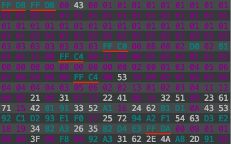
I am using a plugin in IntelliJ called BinEd to view the byte data of the jpeg. I would highly recommend using an editor to view the binary data of the image. It is extremely useful when debugging code.
This is only the first few lines of the byte data of an example image. As you can see, at the start of each segment, there is a marker that starts with an FF byte, followed by a unique byte marking the type of the segment. From the example, there are markers underlined in red; FFD8, FFDB, FFC0 and so on. This is how a JPEG file is laid out, just a long sequence of bytes. Here is a list of the most important markers you’ll need to know about:
0xFFD8 - Start of Image
0xFFE0 - Application Specific (JFIF)
0xFFE1 - Application Specific (EXIF)
0xFFDB - Define Quantization Table(s)
0xFFC0 - Start of Frame (Baseline DCT)
0xFFDD - Define Restart Interval
0xFFC4 - Define Huffman Table(s)
0xFFDA - Start of Scan
0xFFD9 - End of Image
Looking back at the example byte data, the marker FFD8 corresponds to the start of image, which makes sense since it is the first marker of the image. Next there is an FFDB marker which defines a segment of the byte data where one of more quantization tables are stored. FFC0 defines the start of frame for baseline images (note that for progressive images, there will be an FFC2 marker and usually multiple SOS markers identifying the scans). Anyway, I’m sure you get the idea. If ever you run into bugs along the way, a good idea is to come back to these definitions, identify the current segment you are analyzing and identify the bytes you are currently reading. This will be especially helpful when using bit streams to read the scan data.
With a good place to start working from, we can begin by setting up an input stream to read data from the JPEG, byte by byte:
void decode(String image) throws IOException {

    // jpeg image data
    int[] jpegImgData;
    try(DataInputStream dataIn = new DataInputStream(new FileInputStream(image))) {

        List<Integer> d = new ArrayList<>();

        while(dataIn.available() > 0) {
            int uByte = dataIn.readUnsignedByte(); // unsigned byte
            d.add(uByte);
        }

        jpegImgData = d.stream().mapToInt(Integer::intValue).toArray();
    }

    // init values
    qTables = new HashMap<>();
    hTables = new HashMap<>();
    fileName = image.substring(0, image.lastIndexOf('.'));
    mode = -1; // 'uninitialized' value, use first sof marker encountered

    System.out.println("Reading " + image + "...\n");

    // start decoding...
    main: for(int i = 0; i < jpegImgData.length; i++) {
        if(jpegImgData[i] == 0xff) {
            int m = jpegImgData[i] << 8 | jpegImgData[i+1];
            switch (m) {
                case 0xffe0 -> System.out.println("-- JFIF --");
                case 0xffe1 -> System.out.println("-- EXIF --");
                case 0xffc4 -> { // Define Huffman Table
                    int length = jpegImgData[i + 2] << 8 | jpegImgData[i + 3];
                    decodeHuffmanTables(Arrays.copyOfRange(jpegImgData, i + 4, i + 2 + length));
                }
                case 0xffdb -> { // Quantization Table
                    int length = jpegImgData[i + 2] << 8 | jpegImgData[i + 3];
                    decodeQuantizationTables(Arrays.copyOfRange(jpegImgData, i + 4, i + 2 + length));
                }
                case 0xffdd -> { // Define Restart Interval
                    int length = jpegImgData[i + 2] << 8 | jpegImgData[i + 3];
                    int[] arr = Arrays.copyOfRange(jpegImgData, i + 4, i + 2 + length);
                    restartInterval = Arrays.stream(arr).sum();
                }
                case 0xffc0 -> { // Start of Frame (Baseline)
                    int length = jpegImgData[i + 2] << 8 | jpegImgData[i + 3];
                    decodeStartOfFrame(Arrays.copyOfRange(jpegImgData, i + 4, i + 2 + length));
                    if(mode == -1) mode = 0;
                }
                case 0xffc2 -> { // Start of Frame (Progressive)
                    if(mode == -1) mode = 1;
                }
                case 0xffda -> { // Start of Scan
                    int length = jpegImgData[i + 2] << 8 | jpegImgData[i + 3];
                    decodeStartOfScan(
                            /*Arrays.copyOfRange(jpegImgData, i + 4, i + 2 + length),*/
                            Arrays.copyOfRange(jpegImgData, i + 2 + length, jpegImgData.length - 2)); // last 2 two bytes are 0xffd9 - EOI
                    break main; // all done!
                }
            }
        }
    }
}
This will be the entry point for the decoder. The start of the decode method reads all the image data into an array of unsigned bytes. Some values are then initialised that we will be using in later segments. We can start by simply looping over the bytes in this newly constructed array, checking for an 0xFF byte which would mark the start of a new segment. From there we can identify each marker by reading the following byte, and in turn deal with that segment accordingly. Due to how a JPEG is structured, by the time we reach the 0xFFDA Start of Scan marker (which contains the actual image data), we would have already read all other segments we need to begin decoding the scan data. You may notice that in most of the case blocks, there is a length variable as well as a call to copyOfRange(). The two bytes immediately following most markers will signify the length of that segment. Not all markers have this length defined, but most will. The call to copyOfRange() constructs an array from the remaining bytes of that segment. This copied chunk of data is the main payload of that particular segment, and each will be used to extract the relevant information for decoding. This is by no means the most efficient way to unpack bytes of a JPEG, but it is a start.
So far that’s alot of information I’ve thrown at you. But by understanding the structure of a JPEG image, the problem just becomes figuring out what data each segment contains, and how to use it to decode the image. We’ll go through each segment one by one.
Before that though, I’d just like to take a minute to explain a few concepts that you will need to understand about JPEG images before we go on. It may be a helpful to refer back to this section throughout the remainder of this post.
Colour Space Conversion, YCbCr.
The very first step in the encoding process is to convert the RGB pixel values that make up the image into the YCbCr colour space. Made up of three components. Y represents the luminance, or brightness of the pixel. Greyscale JPEG images will be entirely composed of just this brightness information. Cb and Cr make up the chrominance, or colour, part of this trio. They describe the chroma blue and chroma red values for a pixel. Converting images to YCbCr first, allows the brightness and colour of an image to be dealt with separately. This is helpful because brightness information is more important to us in the overall perceptual quality of an image than colour information is. By separating these components into different channels, greater compression can be applied to the colour data, and less so to the brightness data.
Smart, huh? So much thought and ingenuity contained inside the images we see every day. Think about all the JPEG images on the internet! On Wikipedia, there is a paragraph that mentions several billion JPEG images are produced on a daily basis as of 2015!
Anyway, with this knowledge, we can now tackle the concept of chroma subsampling.
Chroma Subsampling and Minimum Coded Units (MCUs)
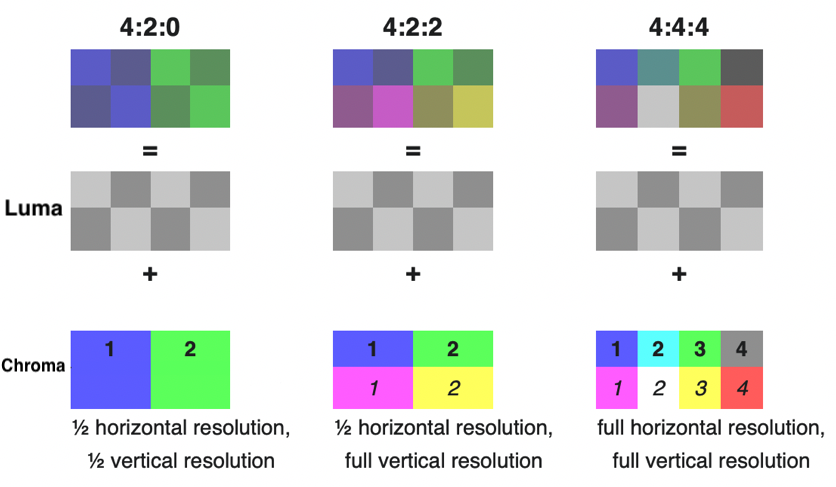
In order to take advantage of the limitations we have when seeing colours, JPEG images will more often than not be chroma subsampled. This lossy compression may produce very significant reductions in file size. The process here involves sampling colour information inside the image at a lower resolution than the luma information. You can think of this as using only the ‘average’ colour of a group of pixels. In order to better understand what that means, let’s look at the three most common types of subsampling:
- 1x1 (4:4:4, no subsampling) - This means there is no subsampling on the image, and colour information is preserved for every pixel.
- 2x1 (4:2:2) - The chrominance components are sampled with half the horizontal resolution in relation to the luminance component. This is the most common type of subsampling you’ll see with digital cameras.
- 2x2 (4:2:0) - The chrominance components are sampled with half both the horizontal, and vertical resolution in relation to the luminance component. This preserves only a quarter of the original colour information.
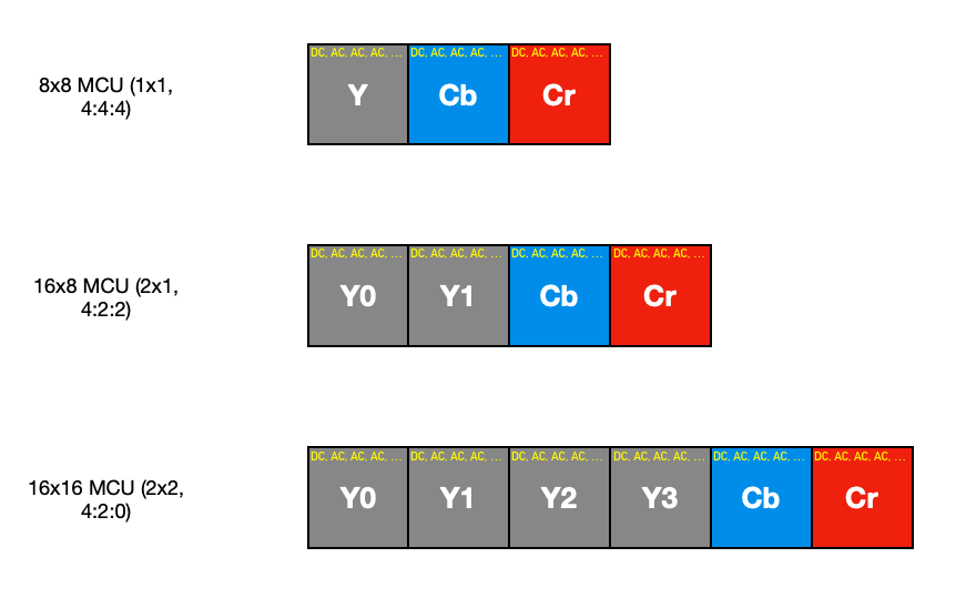
This may be easier to see with the following graphic that I may or may not have stolen (and modified a little) straight from Wikipedia ¯\(ツ)/¯ :
There are other types of subsampling that you may see, including 4x1 (4:1:1), which preserves a quarter of the horizontal resolution, or 1x2(4:4:0), which is sampled with half the vertical resolution. These are much less common though. In fact, the JPEG standard allows for all sorts of strange sampling rates, including the Frankenstein’s monster of them all, Sony’s 3:1:1 sampling rate.
This chroma subsampling that takes place is the reason you may come across minimum coded units, or MCUs, of different sizes. Rather than just performing all encoding or decoding on the entire image all at once, an encoder will divide the image into blocks first called mcus. Usually, without subsampling, these MCUs would be 8 pixels wide, by 8 pixels high. These 8x8 blocks are then processed individually, before moving onto the next block. It is important to make the distinction between these blocks and the MCUs when trying to understand how chroma subsampling affects the MCU size. If there is subsampling of any sort, the MCU size would become a new multiple of these 8x8 blocks. Take 2x1 subsampling for example, the MCU would be 16x8 pixels made up of two horizontal 8x8 luminance blocks, and two 16x8 chrominance blocks (Cb and Cr). In this example, these chrominance blocks are made up of the 8 averaged horizontal pixels, meaning each pair would contain the same colour information. When we start decoding chroma subsampled images, you can treat these 16x8 chrominance blocks just as you would two 8x8 blocks, so no significant changes will have to be made to the decoder.
Huffman Encoding
After the lossy stages of JPEG compression, further encoding will take place following the DCT and quantization steps to represent data in as few bits as possible. A method of entropy encoding known as huffman encoding is one of the final processes that occurs in JPEG compression.
Huffman encoding is a lossless compression method that represents symbols/characters with variable length codes. The length of these codes, or sequence of bits, depends on the relative frequency of the symbol. Put a little more simply, how often a symbol occurs will determine it’s corresponding huffman code. That may sound a little confusing, but we’ll go over a simplified example of this which will hopefully help.
We’ll use the string ‘Hello World’ as our data. If we were to encode this using huffman encoding, we would look at the frequency of each letter/symbol, and assign it a unique code. The code can be of any length, but must not be a prefix of another code. This way, when reading the bit sequence containing the huffman codes, they’ll be no ambiguity about which symbol the code maps to. The following table illustrates this:
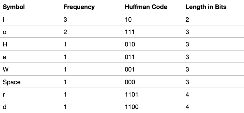
From this table, we can see that our string would map to the bit sequence 01001110101110000011111101101100. In practise, when we get to reading the scan data, we will actually start by building a Huffman tree before hand, but I’ll save that explanation for later.
Discrete Cosine Transform (DCT)
The most important, and maybe the most confusing, aspect of JPEG compression would probably be the Discrete Cosine Transform, or DCT. I touched on this earlier, but now I’ll try to explain what it is and how it works. There is alot to say about this, because it is used in most of the digital media that exists. This includes most formats for images, videos, audio and so on. The DCT is used to represent the sequence of data points that make up an image, as a sum of various cosine functions. Each function will have a unique frequency. You may see this described as a conversion from a spatial domain to a frequency domain, and it allows the image data to be manipulated much more easily for compression. I mentioned earlier that we as humans aren’t great at seeing colours. Well, we also can’t see high frequency variations in brightness very well either, and this conversion allows for specific data to be removed to take advantage of this.
Remember those 8x8 blocks I spoke about earlier? Well, in JPEG, DCT is applied to each of these blocks individually to produce 8x8 coefficient matrices. Each component that makes up one of these matrices will tell us how much of that particular frequency will contribute to reconstruct the original 8x8 image block. If you need to, revisit the second video about JPEG compression by ComputerPhile, it took me a few watches before I really understood this concept.
Here is what the 2D DCT functions matrix looks like:
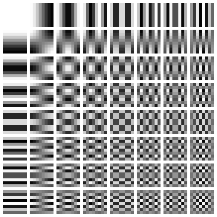
This is the matrix representing the 64 cosine functions that can be combined to form any 8x8 image. Lower frequency information exists in the top left portion of this coefficient matrix, and you’ll find these to be much higher values. Mostly, such a small portion of an image (8x8 pixels) won’t contain a lot of variation, or high frequency information. You may see slight changes in gradient, or a gradual shift between colours, but not much fine detail. Subsequently, this means the higher frequency information that exists in the coefficient matrix towards the bottom right, will have very small values close to 0. These values get rounded to 0 during quantization which is where data is actually deleted from the image, and where one of the lossy parts of JPEG compression occurs. This is how high frequency information in an image is discarded.
With all that out the way, I think it’s probably time to move onto the markers inside the JPEG file, and see what kind of data they contain.
1. Application Specific Marker
We have established JPEG is just a compression method. So what is the file format? Well, the JPEG standard defines how to decode and encode the data, but has no details about the file format used to contain it. So, once upon a time someone somewhere came up with the JFIF standard and everyone just stuck with that. Then there is also EXIF, which is newer and much more commonly used with digital cameras. It stores extra information such as the camera settings used when taking the picture. Some files may even contain both EXIF and JFIF headers. These are the two most common formats, but for the sake of writing a decoder, we don’t need to worry about these differences. Extra metadata about the image stored in this tag won’t affect how we decode the JPEG file. It’s just good to know what they are when you see them. Note that thumbnail image data can also be stored under these segments.
The markers FFE0 through to FFEF are used to identify these app specific segments, and you can read through their structure here:
2. Define Quantization Table(s)
There are two main operations that make JPEG a type of lossy compression. Chroma subsampling is one. The other, is part of the quantization process. During encoding, quantization allows a significant portion of the image data to be discarded without there being much noticeable difference that we can observe. This takes full advantage of how the human eye cannot see colours very well, as well as being less sensitive to high frequency variation in brightness. There will be one or more tables stored in this segment that we will need to extract for the decoding process. I’ll talk through this in more detail when we get to decoding the scan data, but for now let’s look at how to extract the tables.
private void decodeQuantizationTables(int[] chunk) {

    int d = chunk[0]; // 0, 1 - Y, CbCr
    int[] table = Arrays.copyOfRange(chunk, 1, 65); // 8x8 qt 64 values

    qTables.put(d, table);

    int[] newChunk = Arrays.copyOfRange(chunk, 65, chunk.length);
    if(newChunk.length > 0)
        decodeQuantizationTables(newChunk);
}
Remember the chunk of data we copied earlier, well that is exactly what is passed into the decodeQuantizationTables() method. In fact, each dedicated method for decoding a segment will have this chunk array as a parameter. Depending on the segment, this chunk array will itself have a particular structure. In the case of the quantization segment, it’ll look like this:
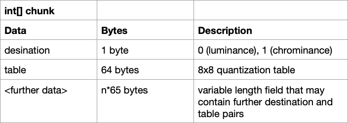
Let’s first discuss what destination means. This destination byte will mark what the quantization table should be used for; 0 for the luminance channel and 1 for the chrominance channel. A JPEG may contain other quantization tables, such as one for the thumbnail image, but we will just be looking for the luminance and chrominance ones. You may not see a chrominance table here if the image is greyscale. After the destination byte, the 8x8, 64 values of the table will follow. In the above code, we extract the destination(d) and those 64 values(table), and put them into a hashmap we can reference later with the destination as the key. Some images may have multiple tables stored under just the one QT marker, that’s what the recursive call at the end is for, to extract any remaining tables.
3. Start of Frame
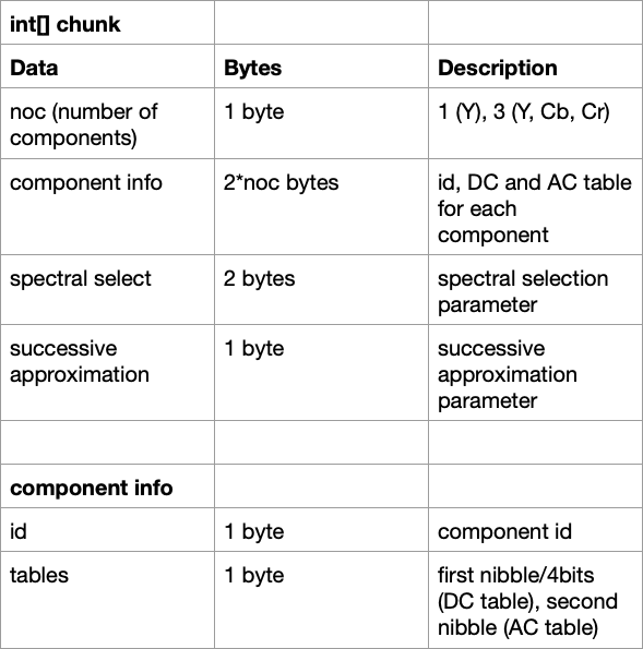
The start of frame segment is the part of the JPEG image were we extract the bit precision, the image width and height, number of components (which would tell us if it is a greyscale image or coloured) and the type of subsampling applied if there is any. It doesn’t take much code to achieve this, but it is important to know which bytes contain this information. Here is the decodeStartOfFrame() method:
private void decodeStartOfFrame(int[] chunk) {
    precision = chunk[0];

    height = chunk[1] << 8 | chunk[2];
    width = chunk[3] << 8 | chunk[4];
    int noc = chunk[5]; // 1 grey-scale, 3 colour
    colour = noc==3;

    // component sample factor stored relatively, so y component sample factor contains information about how
    // large mcu is.
    for(int i = 0; i < noc; i++) {
        int id = chunk[6+(i*3)]; // 1 = Y, 2 = Cb, 3 = Cr, 4 = I, 5 = Q
        int factor = chunk[7+(i*3)];
        if(id == 1) { // y component, check sample factor to determine mcu size
            mcuHSF = (factor >> 4); // first nibble (horizontal sample factor)
            mcuVSF = (factor & 0x0f); // second nibble (vertical sample factor)
            mcuWidth = 8 * mcuHSF;
            mcuHeight = 8 * mcuVSF;
            System.out.println("JPEG Sampling Factor -> " + mcuHSF + "x" + mcuVSF + (mcuHSF==1&&mcuVSF==1?" (No Subsampling)":" (Chroma Subsampling)"));
        }
        // int table = chunk[8+(i*3)];
    }
}
The structure of the chunk of data for this segment (excluding the marker and length of course), looks like this:
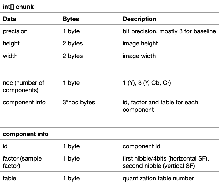
There are a few bitwise/bitshift operations here. Those are just used to combine bytes for the width and height, and find the horizontal and vertical sample factors from the one factor byte. Take note that the colour variable will track whether of not this is a colour image, which we’ll need to know later in decoding the SOS. Also, a JPEG image will store sample factors for each component relatively, so if there is chroma subsampling on the image, you’ll only see the factor for the Y component change. Checking if the id is 1, we can look at just the Y component information and determine the size of the MCU from its horizontal and vertical sample factor.
4. Define Restart Interval
The Define Restart Interval, or as I like to refer to it, the headache segment, is a marker you may see on some JPEG images. Before I knew what this was, I struggled for hours trying to figure out why some images weren’t decoding properly. It was because restart markers existed in the image data. What was even more frustrating was that the solution was extremely simple. JPEG restart markers are designed to allow a resync after an error, as well as enable multi-threaded encoding and decoding, by dividing image scan data up into sections (groups of MCUs). At the start of each section, the DC values have to be reset to 0. I’ll elaborate on this further when we get to decoding the image data, and looking at how the data is laid out, but this would allow each section to be decoded independently. Our decoding is going to be single-threaded though, so we only need to worry about how often these markers occur in the scan data and making sure to reset the DC values when we reach one. To find this interval value (which tells us the number of MCUs between restart markers), we need to look for the FFDD restart interval marker. Let’s take a closer look at the earlier case statement for this:
case 0xffdd -> { // Define Restart Interval
    int length = jpegImgData[i + 2] << 8 | jpegImgData[i + 3];
    int[] arr = Arrays.copyOfRange(jpegImgData, i + 4, i + 2 + length);
    restartInterval = Arrays.stream(arr).sum();
}
Here, there is no dedicated method call to decode this segment, because all the information we need can be found in one line. Two bytes will follow the marker and length that will give us the interval value in MCUs. Taking the sum of this array, and assigning it to restartInterval, we can later count through the MCUs as we decode them.
But what do the restart markers look like? If a restart interval is defined within the image, the scan data will contain various restart markers incrementing from 0xFFD0 up to 0xFFD7, and then starting over again at 0xFFD0.
5. Define Huffman Table(s)
In the earlier section on Huffman encoding, I mentioned that when we begin decoding the scan data, we will first have to construct a Huffman tree. We’ll use this tree to find mappings between the Huffman codes and the components we’ll need. Huffman trees are a type of binary tree (each node only has two children) that contain symbols at the leaf nodes. To reach each symbol, you’d have to traverse down a variable number of branches in the tree, where each branch represents either a 0 or a 1. This can be better illustrated graphically. Let’s take the example string we used earlier, ‘Hello World’. Constructing a Huffman tree from this data would look like this:
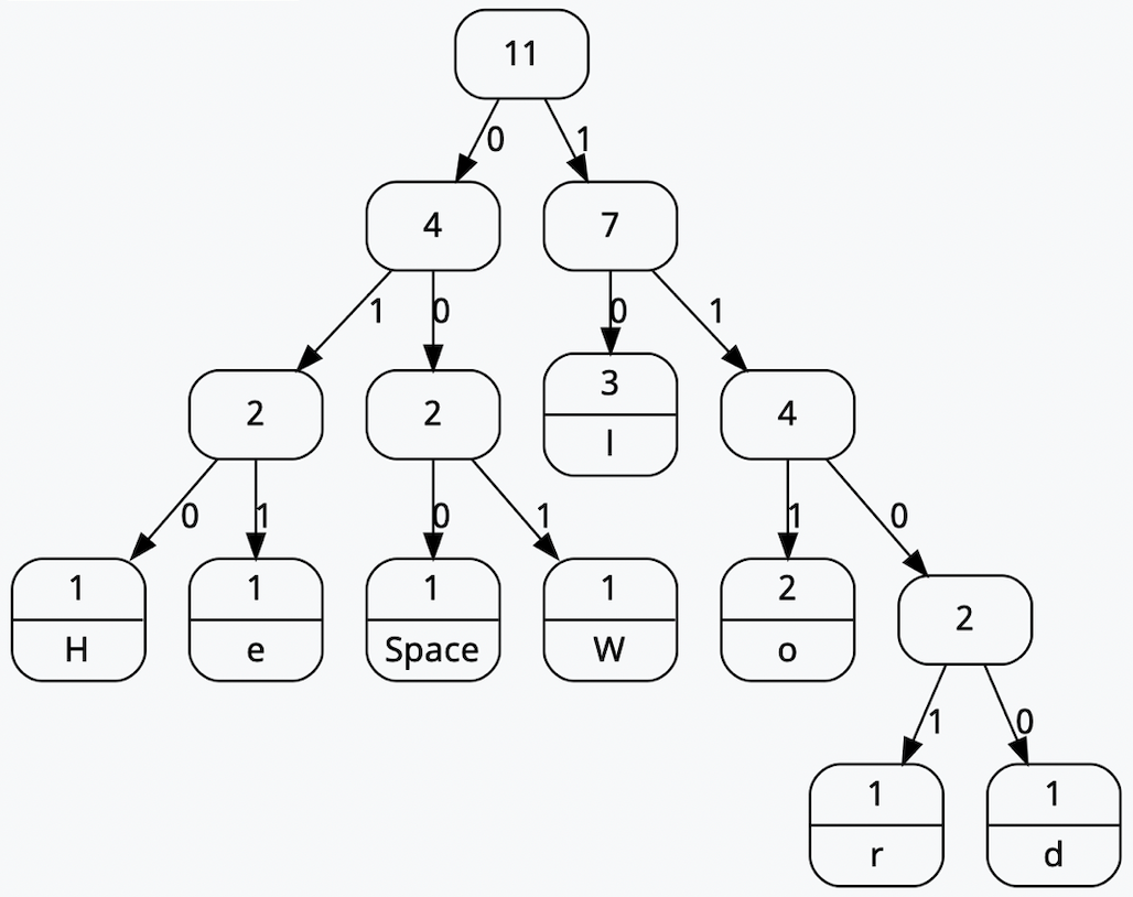
Here, each leaf node contains one of the symbols used in the example String. So, the symbol ‘H’ is encoded by the bit string ‘010’
Decoding the segment of a JPEG that contains these Huffman tables, we will only be given a list of lengths and code values. Therefore, it is up to us to create the huffman tree from this data, prior to decoding the SOS segment, to eventually find the bit string mappings.
private void decodeHuffmanTables(int[] chunk) {

    int cd = chunk[0]; // 00, 01, 10, 11 - 0, 1, 16, 17 - Y DC, CbCr DC, Y AC, CbCr AC
    int[] lengths = Arrays.copyOfRange(chunk, 1, 17);
    int to = 17 + Arrays.stream(lengths).sum();
    int[] symbols = Arrays.copyOfRange(chunk, 17, to);

    HashMap<Integer, int[]> lookup = new HashMap<>(); // code lengths, symbol(s)
    int si = 0;
    for(int i = 0; i < lengths.length; i++) {
        int l = lengths[i];

        int[] symbolsOfLengthI = new int[l];
        for(int j = 0; j < l; j++) {
            symbolsOfLengthI[j] = symbols[si];
            si++;
        }

        lookup.put(i+1, symbolsOfLengthI);
    }

    hTables.put(cd, new HuffmanTable(lookup));

    int[] newChunk = Arrays.copyOfRange(chunk, to, chunk.length);
    if(newChunk.length > 0)
        decodeHuffmanTables(newChunk);
}
This is what the method looks like for extracting the table that we will later use to create the Huffman tree. Here is what the chunk of data will contain:
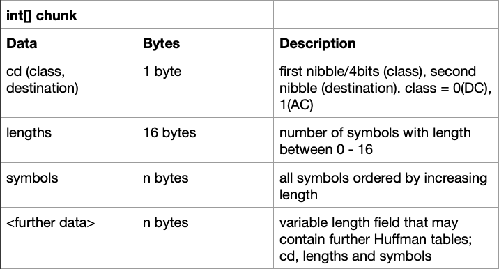
First there is the class and destination, which are each only 4 bits long. The class will mark whether this table should be used for the DC (0) or AC (1) components, and destination marks what channel the table should be used for; 0 for luminance and 1 for chrominance. Reading this as just one byte though, we’ll have four possible options for the cd variable:
- 0 (00) - Table for DC luminance components
- 1 (01) - Table for DC chrominance components
- 16 (10) - Table for AC luminance components
- 17 (11) - Table for AC chrominance components
The lengths field of the chunk will always be 16 bytes long. Each position within this array will correspond to the length of the Huffman code, and the number at that position will indicate how many of those codes with that length there are. That was mouthful, but much like everything in this post, it should be a little easier to understand with an example. Let’s imagine our lengths array looks like this:
[0, 1, 3, 5, 3, 3, 2, 2, 0, 0, 0, 0, 0, 0, 0, 0]
This would tell us that there are 0 Huffman codes with a length of 1 bit. There is 1 Huffman code of length 2 bits, 3 Huffman codes of length 3 bits, 5 Huffman codes of length 4 bits and so on. Taking the sum of this array would tell us the total number of Huffman codes that exist. All the symbol mappings will then follow these 16 bytes. Much like the quantization segment, multiple tables may be stored under just the one marker, so make sure to extract any remaining tables.
In the above decodeHuffmanTables() method, all these variables (cd, length, symbols) are used to construct a HuffmanTable instance. This requires a hashmap containing the code lengths and symbols. From there, the new HuffmanTable is added to the hTables hashmap initialised earlier that’ll be used later when decoding the SOS segment. The final recursive call will find any remaining tables still stored inside the segment.
Let’s pick apart the HuffmanTable class to see what’s going on:
class HuffmanTable {

    private final HashMap<Integer, int[]> lookup;
    private final Node root;

    private static class Node { // node in binary tree

        private int symbol;
        private Node[] children; // children[0] - left child, children[1] right child
        private Node parent;

        private Node() { // root
            symbol = -1; // nodes left with symbol -1 are not leaf nodes, i.e have children
        }
        private Node(Node parent) {
            this();
            this.parent = parent;
        }
        private void initChildNodes() {
            children = new Node[]{new Node(this), new Node(this)};
        }
    }

    HuffmanTable(HashMap<Integer, int[]> lookup) {

        // hashmap reference to code lengths with corresponding symbols
        this.lookup = lookup;

        // construct huffman tree
        root = new Node();
        root.initChildNodes();
        Node leftMost = root.children[0];
        Node current;

        for(int i = 1; i <= lookup.size(); i++) {
            if(getSymbolCount(i) == 0) {
                current = leftMost;
                while(current != null) {
                    current.initChildNodes();
                    current = getRightNodeOf(current);
                }
                leftMost = leftMost.children[0];
            } else { // symbols to put into the nodes of the binary tree
                for(int symbol : getSymbols(i)) {
                    leftMost.symbol = symbol;
                    leftMost = getRightNodeOf(leftMost);
                }
                leftMost.initChildNodes();
                current = getRightNodeOf(leftMost);
                leftMost = leftMost.children[0];
                while(current != null) {
                    current.initChildNodes();
                    current = getRightNodeOf(current);
                }
            }
        }

    }

    private int getSymbolCount(int n) { // # of symbols with length n bits
        return lookup.get(n).length;
    }
    private int[] getSymbols(int n) { // returns list of symbols with length n bits
        return lookup.get(n);
    }
    private Node getRightNodeOf(Node node) {
        if(node.parent.children[0] == node) return node.parent.children[1];
        int traverseCount = 0;

        while (node.parent != null && node.parent.children[1] == node) {
            node = node.parent;
            traverseCount++;
        }

        if(node.parent == null) return null;

        node = node.parent.children[1];

        while (traverseCount > 0) {
            node = node.children[0];
            traverseCount--;
        }

        return node;
    }

    public int getCode(BitStream stream) {
        Node currentNode = root;
        while(currentNode.symbol == -1) {
            int bit = stream.bit();
            if(bit < 0) { // end of bit stream
                return bit; // no more codes to read
            }
            currentNode = currentNode.children[bit];
        }
        return currentNode.symbol;
    }
}
Firstly, there is the lookup hashmap defined at the top of the class. This is the same hashmap that was created and passed into the constructor. Next, the binary Huffman tree is constructed using the Node class. This class will represent a node within the tree and will contain a reference to it’s parent node as well as it’s left and right child nodes. The symbol will contain -1 for nodes that have children (i.e the bit sequence, or path along the branches to that node does not map to any symbol). For leaf nodes, this field will contain the symbol mapping for the given Huffman code. All other methods in the HuffmanTable class are just there to be used in the construction of the tree, with one exception; getCode(). We haven’t discussed the BitStream yet, and we will come back to this method later, but for now, just know that this method is used to traverse the Huffman tree to find the symbol mapping for a given Huffman code.
That’s more or less everything you’ll need to undestand about Huffman encoding. This is definitely another part of JPEG that takes a while to get your head around, but if you’ve made it this far, then you’re probably pretty determined to understand this stuff anyway. If that is the case, then congratulations, you’re now part of the weird group of people that actually care about how JPEG images work. With that being said, we’re not done yet, actually, we’re probably only about halfway through. The final thing we need to do is decode the scan data. But before we get to that, here is a random Monty Python sketch because why not.
6. Start of Scan
So far, everything we have done has just been preperation for this step. Hopefully, this is where everything will become much clearer, and we’ll see how each of the segments we have looked at will play a role in decoding the image scan data. There will be a number of methods and classes we will use here, but just like the other markers, we’ll start at the segment’s dedicated decode method. There is alot going on in this method, so we’ll look at it in parts, starting from the method signature:
private void decodeStartOfScan(/*int[] chunk, */int[] imgData) {}
We are no longer using the chunk array because we don’t really care too much about what the SOS contains, we are only interested in the scan data. The scan data, or entropy coded image data, is the only part of a JPEG without a preceding marker, rather, it immediately follows the Start of Scan. Even though we won’t be using the data contained in this segment, I’ll leave this table here for anyone who is interested. This shows the structure for the chunk of data:
Now, the only parameter passed into the decodeStartOfScan() method is the imgData[] array. This contains all the entropy coded image scan data we’ll need to decode. I have been using the terms DC and AC throughout this post, but I haven’t really explained what they mean. DC, or direct current, refers to the first component of the DCT. It represents an average of all the pixel values in the block. The remaining 63 values of the 8x8 block are referred to as the AC, or alternating current, components. Every DC value in the coefficient matrices of the image, are encoded relative to the preceding block’s DC value. This means most DC components in the image are much closer to 0 which allows for better compression when Huffman encoding is applied. This is because fewer symbols will be used in the resulting Huffman tree.
The order in which blocks that make up the MCU will occur in the scan data depends on the subsampling that has been used. I spoke earlier about how there will be multiple luminance blocks per MCU if there is chroma subsampling present. Well, the ordering of these blocks in the scan data depends on the type of subsampling, but all luminance blocks will come first, followed by the Cb block and then the Cr block. For greyscale images, there would be no chrominance blocks at all. Here is what this looks like:
With all this is mind, as we decode the scan data, we have to make sure to keep track of the preceding block’s value for the DC component, as well as take into account the order in which blocks are encoded. So, moving on to the first part of the decodeStartOfScan() method:
if(mode != 0) {
    System.err.println("This decoder only supports baseline JPEG images.");
    return;
}

System.out.println("Decoding Scan Image Data...");

List<Integer> imgDataList = new ArrayList<>(imgData.length);
for(int b : imgData) imgDataList.add(b);

// check for and remove stuffing byte and restart markers
for(int i = 0; i < imgDataList.size(); i++) {
    if (imgDataList.get(i).equals(0xff)) {
        int nByte = imgDataList.get(i + 1);
        if (nByte == 0x00) // stuffing byte
            imgDataList.remove(i + 1);
        if (nByte >= 0xd0 && nByte <= 0xd7) { // remove restart marker
            imgDataList.remove(i); // remove 0xff
            imgDataList.remove(i); // remove 0xdn
        }
    }
}

// convert back to int[]
imgData = new int[imgDataList.size()];
for(int i = 0; i < imgDataList.size(); i++)
    imgData[i] = imgDataList.get(i);
First, before any decoding takes place, we should check if this is in fact a baseline JPEG image. Next, the stuffing bytes and restart markers are removed from the scan data. Sometimes, the entropy encoded data will need to contain an 0xFF byte. If this is the case, an 0x00 byte will immediately follow to make sure a decoder won’t interpret this as a predefined segment. So, before we do decode anything, we just remove the 0x00 byte because it isn’t actually part of the data that makes up the image. If you remember from the earlier section, I described that the scan data will contain a series of restart markers. We know how often these markers occur as defined by restartInterval we found in the DRI segment, so we can throw these away from the byte data too. Continuing through the decodeStartOfScan() method, we have:
// list of converted matrices to write to file
List<int[][]> convertedMCUs = new ArrayList<>();

// start decoding
int restartCount = restartInterval; // for restart markers, interval obtained from DRI marker
BitStream stream = new BitStream(imgData);
int[] oldDCCoes = new int[] {0, 0, 0}; // Y, Cb, Cr

// matrices
List<int[][]> yMatrices;
int[][] yMatrix;
int[][] cbMatrix = null;
int[][] crMatrix = null;
Here, we start by initializing a list of matrices to store the MCUs of the image. Next we initialize the restartCount from the restartInterval we found earlier. As we decode through MCUs, this counter will decrement and when it reaches 0, we’ll reset the DC components to 0, and restart the bit stream on the next byte boundary. If there is no restartInterval defined in the image, this will be 0, and, well, no harm done I guess. A BitStream is created from the image scan data which I’ll talk about in a moment. An array called oldDCCoes will keep track of the previous block’s DC components for all three channels. Remember how I mentioned DC values are encoded relatively? For the first block, these are all initialized to 0. Next, we define variables for the matrices that will make up one MCU.
Now, we know that in order to map the Huffman codes from the scan data to the symbols, we’ll need a bit sequence that we can use to traverse the Huffman tree. We’ll need to be able to extract a single bit at a time from the bit sequence. In other words, we’ll need a stream of bits; a BitStream!
The BitStream class is simple enough, it just keeps a copy of the image data array, and a marker pointing to the current bit position that’ll increment as more bits are read:
class BitStream {
    private final int[] data;
    private int position; // bit position

    private int cByte; // current byte
    private int cByteIndex;

    private int bit;

    BitStream(int[] data) {
        this.data = data;
        position = 0;
    }

    public int bit() {
        cByteIndex = position >> 3;
        if(cByteIndex == data.length) return -1;
        cByte = data[cByteIndex];
        bit = (cByte >> (7 - (position % 8))) & 1;
        position++;
        return bit;
    }

    // start on byte boundary
    public void restart() {
        if((position & 7) > 0)
            position += (8 - (position & 7));
    }

    public int getNextNBits(int n) {
        int r = 0;
        for(int i = 0; i < n; i++)
            r = r*2 + bit();
        return r;
    }
}
The bit() method returns the bit at the current position in the image data array, or -1 if the end of the bit stream has been reached (no more data to read). If there are restart markers present, we can restart the bit stream on the next byte boundary with the restart() method. Don’t worry too much about getNextNBits() for now, I’ll come back to this later on. For now, let’s look at the final part of decodeStartOfScan():
outer: for(int i = 0; i < (int)Math.ceil(height / (float)mcuHeight); i++) { // cast to float to avoid rounding errors
    for (int j = 0; j < (int)Math.ceil(width / (float)mcuWidth); j++) {

        // mcu
        yMatrices = new ArrayList<>(); // 2x2 - y0 y1 y2 y3 | 2x1 - y0 y1 | 1x1 y0

        // loop to obtain all luminance (y) matrices, which is greater than 1 if there is chroma subsampling
        for(int k = 0; k < mcuVSF; k++) {
            for(int l = 0; l < mcuHSF; l++) {
                yMatrix = createMatrix(stream, 0, oldDCCoes, 0);
                if (yMatrix == null) // end of bit stream
                    break outer;
                else
                    yMatrices.add(yMatrix);
            }
        }

        if(colour) {
            cbMatrix = createMatrix(stream, 1, oldDCCoes, 1);
            crMatrix = createMatrix(stream, 1, oldDCCoes, 2);
            if(cbMatrix == null || crMatrix == null) break outer; // end of bit stream
        }

        convertedMCUs.add(convertMCU(yMatrices,
                cbMatrix,
                crMatrix));

        if(restartInterval != 0) { // dri marker exists in image
            if(--restartCount == 0) {
                restartCount = restartInterval; // reset counter to interval

                // reset DC coefficients
                oldDCCoes[0] = 0;
                oldDCCoes[1] = 0;
                oldDCCoes[2] = 0;

                stream.restart(); // set bit stream to start again on byte boundary
            }
        }
    }
}

createDecodedBitMap(convertedMCUs);
The MCU width and height that we calculated in the SOF segment can be used to tell us how many MCUs exist in the image, this is what the main nested loop is for; to loop over all available MCUs in the image. If an image’s width or height is not perfectly divisible by an the size of an MCU, you’ll find what are called partial MCUs. They just contain a few pixels that are not part of the image, but are there to complete the MCU. They’ll usually just be duplicated rows or columns, but they have to exist so that every MCU can be decoded in the same way. For example, if the width of the MCU is 8 pixels, and the width of an image is 65 pixels, you’ll have 9 MCUs per row, with the 7 columns of that 9th MCU containing data that isn’t part of the image. This can just be cropped out later on, but we have to make sure we decode every MCU there is. That’s what taking the Math.ceil() of the division in the for loops is for.
Next, we’ll just initialize all the luminance matrices, which will be more than one if the image has been chroma subsampled, as well as the chrominance matrices if it’s a colour image. This is where we use that colour variable we defined earlier. Each matrix, or block, is decoded by the createMatrix() method, which will spit back null if the end of the bit stream has been reached, and there are no more blocks to decode. After decoding, each block that forms the MCU is passed into the convertMCU() method, which gives us the final complete block that makes up part of the image. Each block contains all the RGB pixel values of the original image. That’s right! The end is in sight! That list of converted MCUs keeps a store of all of those complete decoded MCUs, ready to be written to a file. Well, you can do whatever you want with these, the point is the list contains the entire decoded image. We’ll take a look at the createDecodedBitmap() method soon to see how a bitmap image can be created from this list! The last part of the loop, just before we move onto the next MCU, involves the restart interval. A check to see if the restartInterval is 0 tells us if there is a DRI marker inside the image. If there is, the restartCount would have been initialized to that value, and we can decrement it. If it reached 0, we reset the counter, reset the DC components to 0 and call restart() on the bit stream.
So, now we’ve reached the brain of the decoder; the createMatrix() and convertMCU() methods. This is where most of the heavy lifting happens, and we get to actually decoding the 8x8 blocks. Let’s tackle these two methods separately. First, the createMatrix() method:
// key used for dc and ac huffman table and quantization table
private int[][] createMatrix(BitStream stream, int key, int[] oldDCCoes, int oldDCCoIndex) {}
This method takes in the BitStream created from the scan data, a key, that we’ll use to determine which quantization and Huffman tables to use, as well as a reference to the previous block’s DC coefficient (which will be updated from within the method). A call to createMatrix() will return the complete decoded 8x8 block by reversing the Huffman, run-length and zigzag encoding, quantization and DCT. Much like with the SOS segment, let’s look at each step in parts:
DCT3 inverseDCT = new DCT3(precision);
The first line in the createMatrix() method involves creating a DCT3 instance. This is the inverse of the DCT-2 function used by JPEG images. There are many variations of the DCT but for now we only care about DCT-3, or as I’ll be referring to it from now on, the inverse DCT. We extracted the bit precision back in the SOF, and that’s the value passed into the constructor. The DCT3 class does also contain some functionality unrelated to the inverse DCT, but I’ve left it with it’s current name for simplicity’s sake. Here is the class:
class DCT3 { // inverse dct

    private final int[] components;
    private final int[][] zigzag;
    private final int precision;

    DCT3(int precision) {
        components = new int[64];
        zigzag = new int[][] {
                {0, 1, 5, 6, 14, 15, 27, 28},
                {2, 4, 7, 13, 16, 26, 29, 42},
                {3, 8, 12, 17, 25, 30, 41, 43},
                {9, 11, 18, 24, 31, 40, 44, 53},
                {10, 19, 23, 32, 39, 45, 52, 54},
                {20, 22, 33, 38, 46, 51, 55, 60},
                {21, 34, 37, 47, 50, 56, 59, 61},
                {35, 36, 48, 49, 57, 58, 62, 63}
        };
        this.precision = precision;
    }

    public void setComponent(int index, int value) {
        components[index] = value;
    }

    public void zigzagRearrange() {
        for(int x = 0; x < 8; x++) {
            for(int y = 0; y < 8; y++) {
                zigzag[x][y] = components[zigzag[x][y]];
            }
        }
    }

    public int[][] dct3() {
        int[][] matrix = new int[8][8];
        for(int i = 0; i < 8; i++) {
            for (int j = 0; j < 8; j++) {
                matrix[i][j] = j;
            }
        }

        // naive 0(n^4) - decoding high resolution jpg images will take a while
        for(int x = 0; x < 8; x++) {
            for(int y = 0; y < 8; y++) {
                int s = 0;
                for(int u = 0; u < precision; u++) {
                    for(int v = 0; v < precision; v++) {
                        s += (
                                zigzag[v][u]
                                * ((u==0?1.0f/Math.sqrt(2):1.0f) * Math.cos(((2.0 * x + 1.0) * u * Math.PI) / 16.0))
                                * ((v==0?1.0f/Math.sqrt(2):1.0f) * Math.cos(((2.0 * y + 1.0) * v * Math.PI) / 16.0))
                        );
                    }
                }
                matrix[y][x] = Math.floorDiv(s, 4);
            }
        }

        return matrix;
    }
}
The components array will hold all the 64 values of the 8x8 block, and we’ll later use the zigzag 2d array to rearrange these components into a matrix. The dct3 method is where the inverse DCT algorithm is implemented. Now, those four nested loops may make you cringe, which is a perfectly reasonable reaction. There are of course optimizations on this algorithm that will improve efficiency, but I figured for this blog post I’ll leave that up to you! Just be aware that this algorithm will take a little while to decode larger images. Anyway, moving on from that monstrosity, another part of the encoding that takes place after quantization is zigzag encoding. The result of quantizing the values inside the matrix after DCT will leave a lot of zeros towards the bottom right. Remember this is where alot of the high frequency information exists. Well, this can be represented in one long sequence of component values by ordering them in this zigzag fashion:
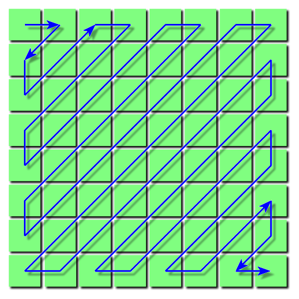
Yes… this is another graphic I swiped from Wikipedia, but I did at least try to create a version of it myself. It looked pretty botched though, so I just went with this. Anyway, you can probably imagine how the sequence we’ll end up with will have all these zeros at the end. This is a simplified example:
15, 14, 12, 9, 9, 9, 8, 8, 4, 3, 2, 2, 0, 0, 0, ..., 0
Run-length encoding compresses data like this really well, and it’s actually the next step that follows this zigzag encoding. The zigzag encoding just prepares the data in the matrix into a sequence so that it can be more effectively compressed with RLE. The RLE expresses those runs of repeated values as two numbers; the data and a count. As we decode, we’ll have to first reverse this RLE and then rearrange the data back into a matrix (undo the zigzag encoding using the zigzagRearrange() method).
With that out the way, let’s see what the next part of the createMatrix() method contains:
int code = hTables.get(key).getCode(stream);
if(code == -1) return null; // end of bit stream
int bits = stream.getNextNBits(code);
oldDCCoes[oldDCCoIndex] += decodeComponent(bits, code);
// oldDCCo[oldDCCoIndex] is now new dc coefficient

// set new dc value to old dc value multiplied by the first value in quantization table
inverseDCT.setComponent(0, oldDCCoes[oldDCCoIndex] * qTables.get(key)[0]);
With all the above in mind, we can finally start looking at the Huffman codes in the scan data. We’ll retrive the Huffman table from the key passed into createMatrix(). This will be 0 for luminance blocks, and 1 for chrominance blocks. Now that we know what the bit stream is, it should be clearer what getCode() of the HuffmanTable class does. It reads individual bits from the BitStream object, and traverses down the tree until it finds a symbol at a leaf node. What exactly is this symbol though? This symbol actually represents a code value, which we’ll use to extract a specific number of bits after the code. These extra bits will represent the signed value of the component we are looking for. Note that the check to see if the code is -1 just tells us if the end of the bit stream has been reached. The getNextNBits() of the BitStream extracts these additional bits. Now, we have two variables; ‘code’ representing the number of allocated bits (or size), and ‘bits’ representing those additional bits. These are the only two things we’ll need to determine the signed component value for this block using the decodeComponent method():
private int decodeComponent(int bits, int code) { // decodes to find signed value from bits
    float c = (float) Math.pow(2, code-1);
    return (int) (bits>=c?bits:bits-(c*2-1));
}
Now, we just increment the old block’s DC component by the newly decoded DC component. Next, we reverse the quantization. Let’s talk about this for a minute.
I’ve spoken about how data is removed from a JPEG during quantization in the encoding process, but how does that happen? After the DCT, each component will be divided by it’s corresponding value in the quantization table. The quantization tables play a big role in reducing file size because they control compression ratio. Let’s take this coefficient matrix as an example (again, thanks Wikipedia):
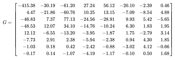
And this quantization table…
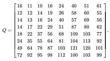
We get…
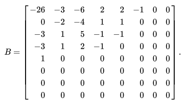
If we take -415.38, divide it by 16 to get -25.96 and round it to -26, we’ll have our DC coefficient for that block. Do you notice how the upper left portion of the quantization table contains smaller values that those towards the bottom right? That’s because those larger numbers will result in divisions closer to 0, in turn producing greater compression. Then, most of those numbers are rounded to 0. This is how the high frequency data is thrown away through lossy compression. Now, after that rounding takes place, we have no way of ever retrieving that data back, because we don’t know what that number was. So, all we can do is multiply each coefficient by its corresponding value in the quantization table to find a close approximation. That’s what we’re doing in the code above. Then this value is set as the first component of the DCT3 class with setComponent().
Here is the next part of the createMatrix() method:
int index = 1;
while(index < 64) {
    code = hTables.get(key+16).getCode(stream);
    if(code == 0) {
        break; // end of block
    } else if(code == -1) {
        return null; // end of bit stream
    }

    // read first nibble of each code to find number of leading zeros
    int nib;
    if((nib = code >> 4) > 0) {
        index += nib;
        code &= 0x0f; // chop off preceding nibble
    }

    bits = stream.getNextNBits(code);

    if(index < 64) { // if haven't reached end of block
        int acCo = decodeComponent(bits, code); // ac coefficient
        inverseDCT.setComponent(
                index,
                acCo * qTables.get(key)[index]);
        index++;
    }
}
This whole section is dedicated to the AC components of the block. Much of the same thing is happening, except we are now using different tables. If the result of getCode() from the HuffmanTable returns a 0, we have reached an EOB, or end of block. This would signify that no more codes exist for the AC components, or in other words, the remaining components are 0. Since values in the components array are assigned 0 initially, we can just move on to the next block if that’s the case. Before we obtain the additional bits, we should also read the first four bits from the code to find the number of leading zeros (this is the RLE). With this, we’ll just skip over those components. Before finding and setting the signed value for the component, we just check we haven’t exceeded the component index of the block (index is less than 64). This leaves the final part of createMatrix():
inverseDCT.zigzagRearrange();
return inverseDCT.dct3();
With the complete list of components in the block, we can now call zigzagRearrange() to form the 2d array, or matrix, and then perform the inverse DCT on the block. This final matrix is returned by createMatrix().
Nice! That covers the most important method in the decoder. Now, all we have to do is convert these matrices for the Y, Cb and Cr channels into one RGB matrix containing the pixel colour values. This is done inside convertMCU(), let’s take a look:
private int[][] convertMCU(List<int[][]> yMatrices, int[][] cbMatrix, int[][] crMatrix) {
    // int values representing pixel colour or just luminance (greyscale image) in the sRGB ColorModel 0xAARRGGBB
    int[][] convertedMCU = new int[mcuHeight][mcuWidth];

    for(int r = 0; r < convertedMCU.length; r++) {
        for(int c = 0; c < convertedMCU[r].length; c++) {

            // luminance
            int yMatrixIndex = ((r/8)*(mcuHSF))+(c/8);
            int[][] yMatrix = yMatrices.get(yMatrixIndex);
            int y = yMatrix[r%8][c%8];

            float[] channels; // rgb or just luminance for greyscale
            if(colour) {
                // chrominance
                int cb = cbMatrix[r/mcuVSF][c/mcuHSF];
                int cr = crMatrix[r/mcuVSF][c/mcuHSF];

                channels = new float[] {
                        ( (y + (1.402f * cr)) ), // red
                        ( (y - (0.344f * cb) - (0.714f * cr)) ), // green
                        ( (y + (1.772f * cb)) ) // blue
                };
            } else {
                channels = new float[] { y };
            }

            for(int chan = 0; chan < channels.length; chan++) {
                channels[chan] += 128; // shift block

                // clamp block
                if(channels[chan] > 255) channels[chan] = 255;
                if(channels[chan] < 0) channels[chan] = 0;
            }

            convertedMCU[r][c] = 0xff<<24 | (int)channels[0]<<16 | (int)channels[colour?1:0]<< 8 | (int)channels[colour?2:0]; // 0xAARRGGBB
        }
    }
    return convertedMCU;

}
Here, the various decoded blocks are converted into one MCU containing pixel values for the image. Should there be subsampling present, the yMatrices list will contain more than one block, and so we have to make sure to obtain the appropriate value for the Y component. Y, Cb and Cr are found for each pixel of the block, and converted to the RGB colour space. Before the DCT can be applied during encoding, all the values in the block are shifted down by 128. This is because the colour values range from 0 to 255. Subtracting 128 just centers those values around 0, because the cosine function ranges from -1 to 1. This is just a preparatory step for the DCT, so when decoding, we just have to shift the block back to the 0 to 255 range by adding 128 to every value. We also just check no values fall slightly outside this range after the shifting, and clamp them to the appropriate limit or minimum if they do. Each value is now stored in the convertedMCU matrix in the ARGB format.
That’s the entire decoding process finished! We obviously want to see what this looks like, and we can do this by creating a bitmap file to store this data:
private void createDecodedBitMap(List<int[][]> rgbMCUs) {
    // prepare BufferedImage for writing blocks to
    BufferedImage img = new BufferedImage(width, height, BufferedImage.TYPE_INT_RGB);

    // set buffered image pixel values for every matrix
    int blockCount = 0;
    for(int i = 0; i < (int)Math.ceil(height / (float)mcuHeight); i++) {
        for (int j = 0; j < (int)Math.ceil(width / (float)mcuWidth); j++) {
            for (int y = 0; y < mcuHeight; y++) { // mcu block
                for (int x = 0; x < mcuWidth; x++) {
                    try {
                        img.setRGB((j * mcuWidth) + x, (i * mcuHeight) + y, rgbMCUs.get(blockCount)[y][x]);
                    } catch (ArrayIndexOutOfBoundsException ignored) {
                    } // extra part of partial mcu
                }
            }
            blockCount++;
        }
    }

    // write bmp file
    try {
        ImageIO.write(img, "bmp", new File(fileName+".bmp"));
        System.out.println("Successful Write to File");
    } catch (IOException e) {
        System.err.println("Error Writing to BMP File. " + e.getLocalizedMessage());
    }
}
This is also where those partial MCUs I spoke about earlier get cropped out. This method just loops through all those decoded MCUs, setting the individual pixel values of a BufferedImage object which gets written to a file.
AND NOW WE’RE FINISHED! Let’s take a look at our results:
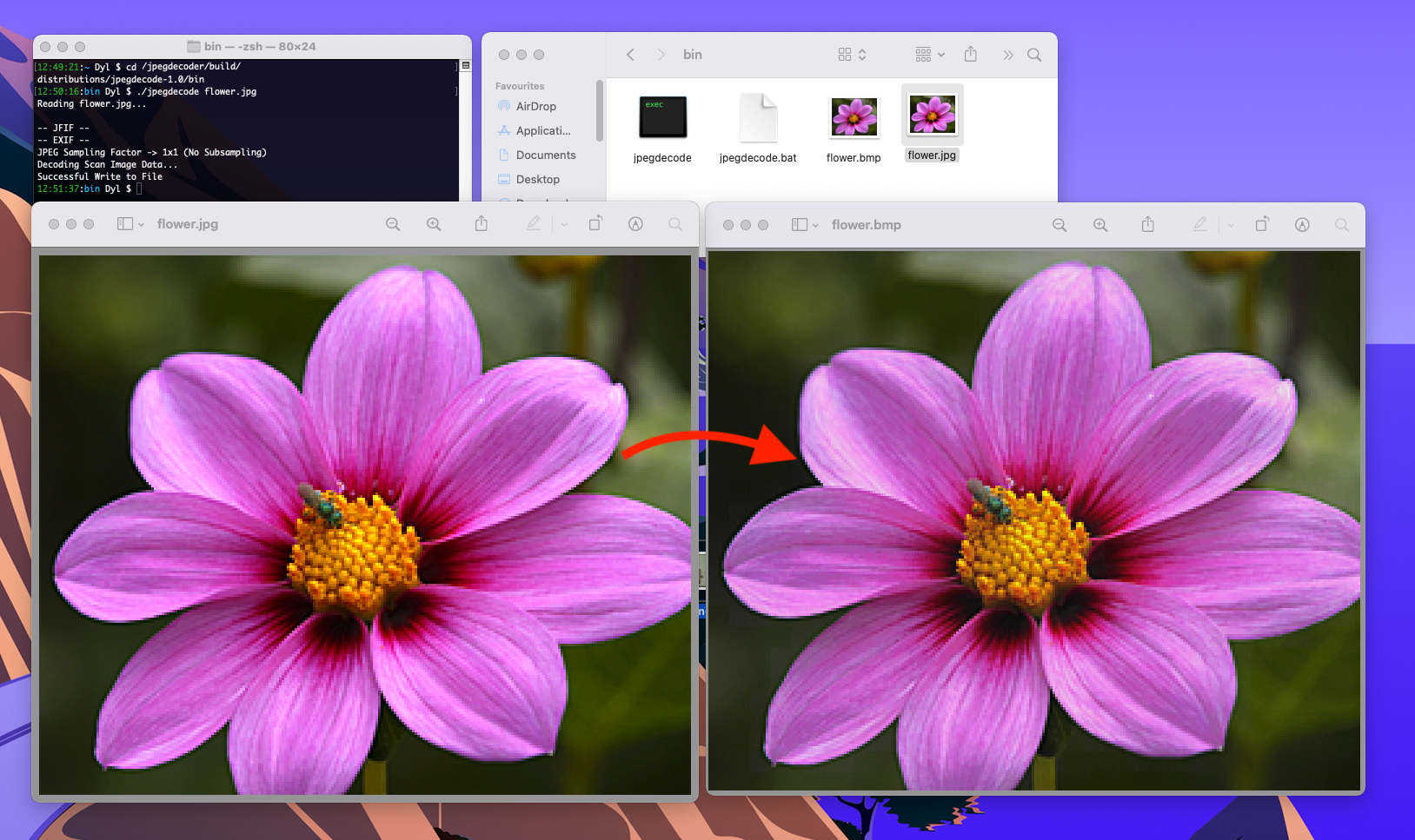
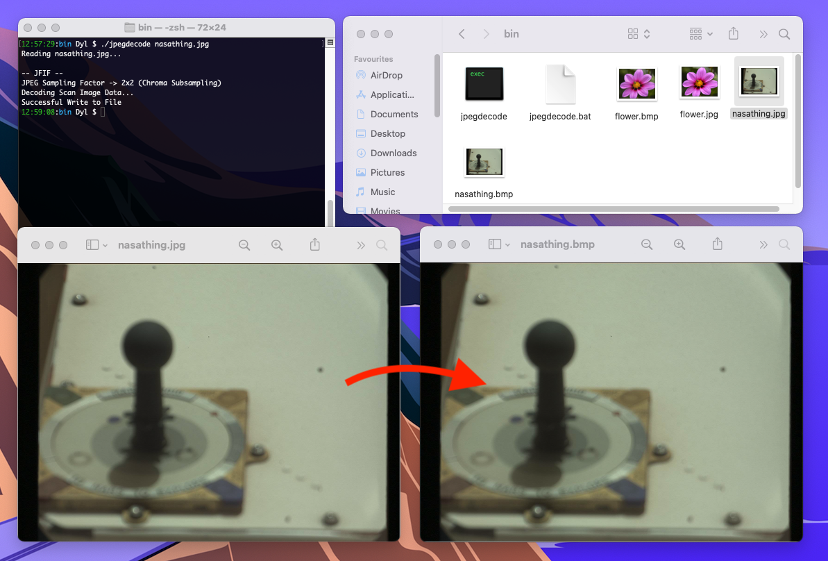
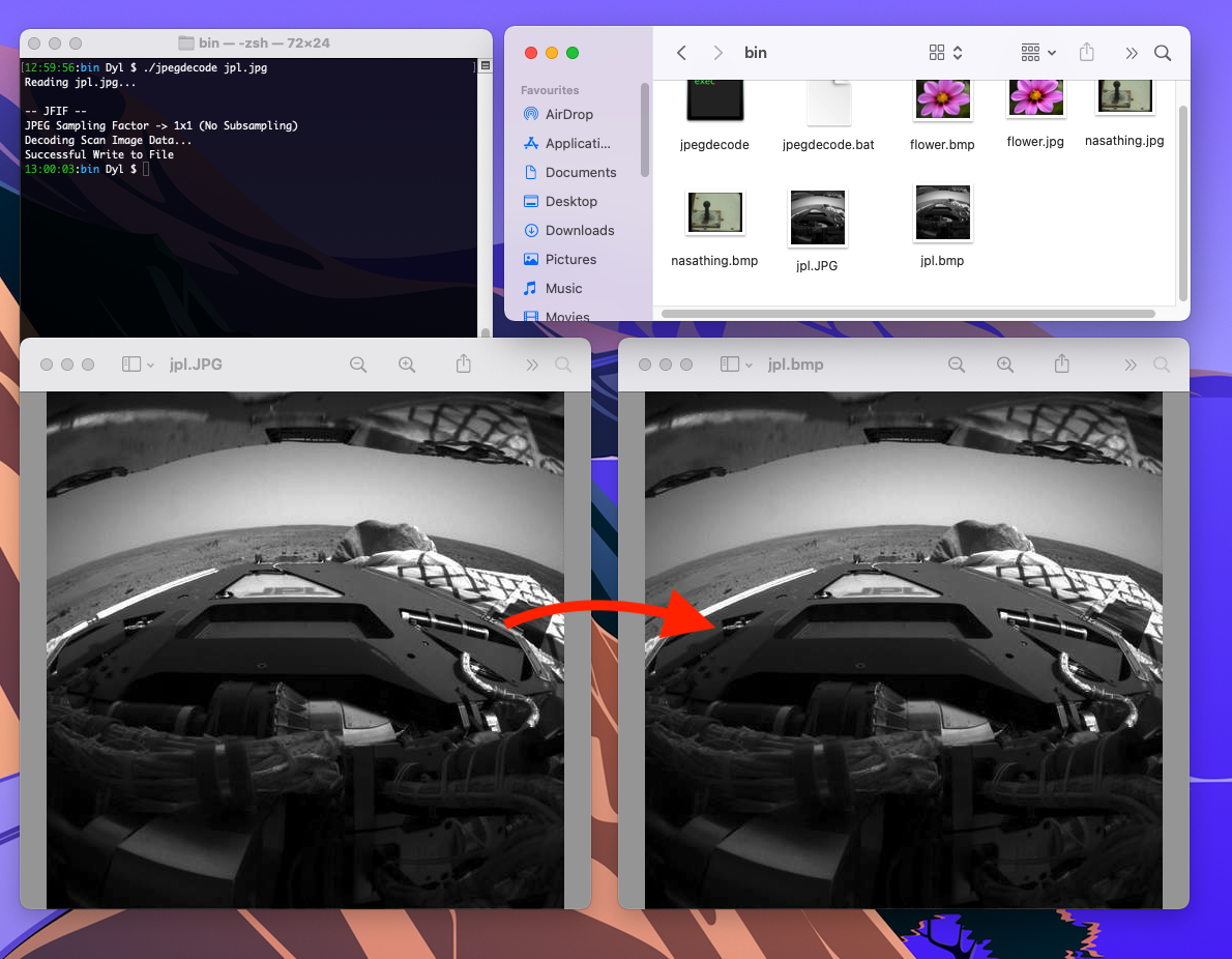
Nice.
Conclusion and Further Reading
That’s it! I hope you found this post helpful. You can find the full source code for this project here. While I did try to be as comprehensive as I could, chances are I may have skimmed over some details. So, if you have any questions or would just like to get in touch, you can email me at dylanlucas1510@gmail.com. Here are some helpful links/resources for further reading:
- JPEG - Wikipedia
- ImpulseAdventure (extremely helpful, see the Technical Articles on JPEG)
- Handy Stack Overflow answer on chroma subsampling
- Github notes on JPEG (there are some helpful diagrams on this page)
Thanks for reading.